GSoC/2021/StatusReports/PhuocKhanhLE

Digikam: Image Quality Sorter Improvement

Image Quality Sorter is a tool of digiKam. It helps users to label image by accepted or pending or rejected. However, the current implementation does not have a good performance. My proposal provides my perspective to improve this functionality.

Mentors : Gilles Caulier, Maik Qualmann, Thanh Trung Dinh

Important Links

Project Proposal

Digikam Image Quality Sorter

GitLab development branch

gsoc21-image-quality-sorter

Project Report

Community Bonding

Community Bonding is the for time for preparation. I spend my first post to describe this important period. Thanks to mentors Gilles Caulier, Maik Qualmann and Thanh Trung Dinh for helping me prepare for the work this summer.

I have spent these 3 weeks reading the huge codebase of digiKam, preparing environment for coding, and study in depth the algorithm that I am about to implement. This is the branch that will have my work for GSoC21.

After reading enough documentation and mathematic, I start preparing a base for testing each functionality of Image Quality Sorter (IQS). I found that it is the most important task in this period. This helps me having a tool to evaluate my future work without thinking further how to test it. There are 2 types of unit test : unit test for each factor (for example : detectionblur) and unit test by pre-defined use-case.

Although these tests can not be passed now, it will be useful in the future.

Blur detection (first week : June 07 - June 14)

The figure below designs my algorithm.

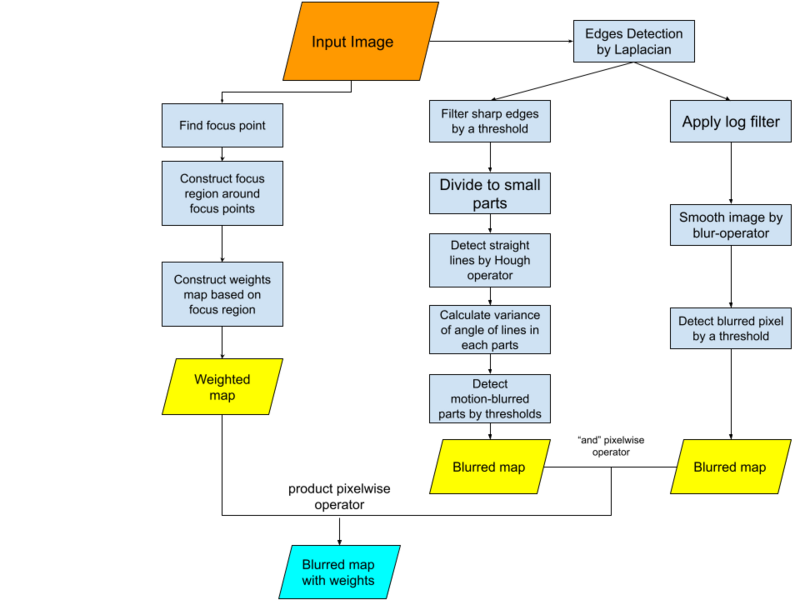
As discussed in the proposal, there are 2 types of blur : motion blur and defocused blur. Hence, there should be detectors for each one due to the difference between their nature. Defocused blur appears when the edges of object are fuzzy. While motion blur appears when the object or the camera moves when capturing.

As observation, I found that defocused blur is the disappearance of edges, while motion blur is the appearance of many parallel edges in a small part of image. Based on algorithm of edges detection Laplacian of opencv, I extract an edges map of the image. I used this map tp detect defocused blur and motion blur of the image.

The advantage of Laplacian is its sensitivity. It detects not only main edges but also the small edges inside the object. So, I can distinguish sharp region belonged to the object and blurred region of background.

Defocused detector :
- This edges map is not enough to detect defocused blur. In order to distinguish sharp pixel of edges and blurred pixel, I apply an log filter. (parameter : ordre_log_filtrer).
- Then, I smooth image by the operateur blur and medianblur of open cv to get a blurred map.
- At last, I determine if a specific pixel is blur nor sharp by using a threshold. (parameter : filtrer_defocus).
Motion blur detector :
- At first, I consider only the clear edges from edges map, by using a threshold. (parameter : edges_filtrer).
- Then, the image is divided into small parts with a pre-defined size (parameter : part_size_motion_blur).
- Then, I apply Hough Line Transform to determine every line in the part. This transformation uses parameter theta_resolution and threshold_hough to find line in an image. Besides, instead of using class Hough transform (cv::HoughLines() ), I use Probabilistic Hough Line Transform (cv::HoughLinesP). HoughLinesP uses more criteria to determine a line than HoughLines includes : min_line_length. This parameter helps to prevent too short line.
- Having lines of a part, it is easy to calculate the angle of them. As mentioned in the proposal, a small part with many parallel lines is a motion blurred part. The parameter min_nb_lines is used to determine if a part can be motion blur. Then, I check if these lines are parallel. There are some tricks to do it :
  - At first, angle alpha and alpha +/- pi are the same in the term of parallelism. Hence, I limit the angle from 0 to pi radian.
  - Secondly, 2 parallel lines have not necessarily same angle degree, but a very proximate value. Hence, I calculate the standard deviation of angle values and compare it to parameter max_stddev. If it is smaller, then, the part is motion blurred.
  - At last, this trick has a weakness when the direction of motion is horizontal. That means angles are around 0 and pi, so the variance would be very big while the image is motion blurred. My solution is to bound the interval of angle only from 0 to (pi - pi / 20). It would solve this case but it is not the best solution.

I tested with test images in unit test of digikam. These images are some different use-cases for blur detection. For instance, the algoritm can recognize the sharp image like rock, or even difficult case like tree. It is also success to recognize motion blur by cheking on image like rock_2 or tree_2. However, the recognition is not very sensitive to jugde them as rejected but only pending.

However, there are still some hard situations. Image street is easy to be recognized as motion blurred because of it nature. Image sky is recognized as defocused blur because of its part sky and cloud.

The project should cover also the artistic image which focus on some specific position and blurs the rest on purpose . It demands an implementation of focus region extractor based on metadata. Moreover, as mentioned above, there is a dead case for the algorithm when the image have background (sky, wall, water, ...). It is reasonable because background doesn't have edges to detect. It also can not be seen as an blurred object. I will try to recognize this part in the next week.

Focuspoint extraction and completion of blur detection (second week : June 14 - June 21)

Camera can use some points (name auto focus points) on image to make the region around sharper. Besides, it blurs the futher region, in order to make an aristic product. These points are named af points. An af point can be pre-defined by camera or by user, depend on model of camera. There are only 2 cases for af points : infocused and selected. Infocues points are the points sharpenned by camera, when selected points is the points expected to be clear by user.

An point can be both in 2 cases (infocus-selected) or neither both (inactive).

Being inspired by the plugins of focus points from LightRoom, I implemented the class FocusPointExractor in the library of metaengines of digiKam. By using exiftool which has been alread deployed in version 7.2 of digiKam, I can easily extract the auto focus infomation (af point). However, there is no standardized document. Therefore, each model of camera has its own function of extracting af points.

Currently, there are 4 models of camera which are extractable for af points :

Nikon
Canon
Sony
Panasonic

Each point is not only a point on the image but a rectangle. Therefore, there are 4 properties : coordinates of center of the rectangle, width, and height. At last, the type of point is the fifth property.

FocusPoint is used to recognized focus region of image. This is a region where user expected to be clear. Therefore, I extract only selected points. For each point, I define focus region is the region around and propotional to the rectangle of point. I consider only pixels within this region for blur detection.

As mentioned in the last week, the algorithm should not consider the region of background, even in the image without focus point. By observation, these regions often have mono-color. Therefore, I detect them by dividing image small part, and calculate the standard deviation of color in this path. If it is smaller than a threshold (parameter : mono_color_threshold), I judge it a part of background and no longer consider it. By this adjustment, the figure below designs the last version of my algorithm.

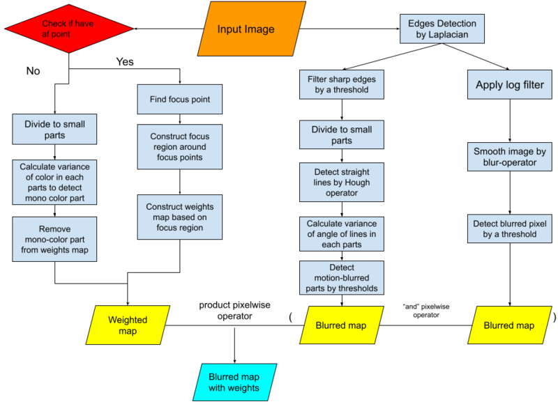
The main problem now is fine tunning the parameter. If I set ordre_log_filtrer and filtrer_defocus too high, the sharp image can be judged pending. Though, If I set them too small, the blurred one can be judged pending.

Noise detection (third and fourth week : June 22- July 04)

Noise detection is implemented base on the paper noise estimation by kurtosis projection. The main idea is to define noise as a random variable followed Gaussian noise. The algorithm estimates the variance of this variable as the level of noise. By using band-pass filter transforms Haar, I can approximate the noise of image to Gaussian noise.

At the end of the algorithm, the result indicates the level of noise. However, it is expected to belong the interval [0 - 1]. However, the variance of noise can vary from 0 to infinity. Therefore, I use sigmoid function to normalize the result. By using to parameter alpha and beta, I can define a sensitive interval of variance. Image with variance at the begin of the interval would be labeled accepted while image with variance at the end of the interval would be labeled rejected.

To test the algorithm, I use some different use-case of noise:

At first, the most common cause of noise is the wrong configuration of ISO parameter in the camera. I use book 1 and graffi 1 as good configuration of ISO, compare to book 2 and graffi 2 as bad configuration of noise. It passes this test on distinguishing these two cases.
Secondly, I test on images with increasing amount of noise from test noised 1 to test noised 9. It passes the test by labeling test noised 1 as accepted, test noised 5 as pending and test noised 9 as rejected.
At last, the detection should detect different kinds of noise. Follows the paper different kinds of noise, I generate noised images from a good image, and test with each case. For now, only noise salt & pepper and noise structure are not yet recognized by the algorithm

Exposure detection and Compressed detection (Fifth week : July 05 - July 11)

Exposure detection

The main idea is using the histogram of luminance of image. I consider number of pixel in only 4 intervals [0 - threshold_underexposed],[threshold_underexposed - threshold_demi_underexposed],[threshold_demi_overexposed - threshold_overexposed],[threshold_overexposed - 255]. Each interval is attached to a weight which present its influence to the image. By using the following expression, I can indicate the level of overexposure and and underexposure of image:

overexposed_level = (over_exposed_pixel * weight_over_exposure + demi_over_exposed_pixel * weight_demi_over_exposure) / (normal_pixel + over_exposed_pixel * weight_over_exposure + demi_over_exposed_pixel * weight_demi_over_exposure)
underexposed_level = (under_exposed_pixel * weight_under_exposure + demi_under_exposed_pixel * weight_demi_under_exposure) / (normal_pixel + under_exposed_pixel * weight_under_exposure + demi_under_exposed_pixel * weight_demi_under_exposure)

At last, I configure the parameters to covers as much as possible user-cases. As image is rarely overexposed underexposed at the same time, I get over/underexposed level is the max between overexposed_level and underexposed_level.

I tested with various situations :

Firstly, the algorithm can distinguish clearly overexposed / underexposed image.
Then, the algorithm can also recognize backlight image as bad image (rejected label).
At last, in some case of artistic work like sun image , the algorithm can only label it as pending.

Compression detection

At first, by studying the algorithm of compression, a compressed image will have an amount of pixel-blocks (as the left half of follow picture) which will reduce the quality of image.

A block is a square mono-color. My algorithm tries to detect the region of all pixel-blocks. I detects 2 types of pixel : pixel inside the block and pixel at the edges of each block:

Inside a block, all pixels have exactly same colors.
I detect pixel at the edges of a block by using this algorithm

Then, I count the number of each one and attach to a weight as parameter. At last, I configure the parameter to fix test-case. Image from test compressed 1 to test compressed 9 is a good example. Test compressed 9 is the original image (2.2 MB) and test compressed 1 is fully compressed (214 KB). For now, the algorithm can label test compressed 9 'accepted' and test compressed 1 as 'pending' ( with very low score of quality).

Calculation of quality and optimization (Sixth and Seventh week : July 12 - July 25)

The result of each quality detection only presents the influence of one aspect on the image. However, quality score is the result of a combination of divers detection. In addition, due to the perspective of users, each quality has a different weight on the quality. Therefore, I make a class of `image quality calculator` to gather the result of each detector and its correspondent weight. The calculator normalizes the weight of each detector to ensure that the result will be in the interval 0 to 100.

In order to test the performance of my algorithm, I use the database KonIQ-10k. Its advantage is that the quality of all images are scored by reliable quality ratings from many crowd workers and include in the interval of 0 to 100 which is suitable to our case. To perform a unit test for the whole `Image quality sorter` (IQS), I create 5 test cases based on five intervals of score in the database: bad image (score : 0 - 10), quite bad image (score: 10 - 30), normal image (score: 30 - 50), quite good image (score: 50 - 60) and good image (score > 60). For each test case, I take from the database 6 images which the correspondent score. Bad and quite bad images would be labeled REJECTED, normal images with PENDING and the last test case would be labeled ACCEPTED. The result is quite promising while it can give the right label on more than half of test-images. However, there are still various fail cases. One of the main reasons is that when an aspect of quality is extremely poor, people will rate it a bad image in spite of the other quality is good. I apply a trick to cover these cases. When a score of an aspect is extremely low, the final quality will get a punish to downgrade the score. This trick works well while it can cover more use-cases.

After having a quite good performance of accuracy, my work continues in optimizing the run-time of IQS. The main idea is to extract the common processes 4 detections and execute it only one time. Then, by applying multi-thread on 4 detections, I can decrease more time of processing.

UI for adding customized focus point and showing focus point (Eighth and ninth week : July 25 - August 9)

One of purpose of this project is to cover artistic image with blurred background. The applied technique is to extract auto-focus point (af point) of camera read from exiftool metadata. However, it is impossible to apply this technique if the image doesn't have auto-focus point or the model of camera is not included in auto focus point extractor. To get around these cases, I make to feature allowing user to create a customized focus point on the image which doesn't this such information.

After adding this feature, it is reasonable to add feature of showing all focus points of an image. As there are 4 types of focus points : inactive, selected, infocus and selected-infocus, I make a separation between them : red rectangle for selected point, green for infocus point, blue for selected-infocus point, and black for inactive point. This feature will prioritize visualize focus point extracted from metadata exiftool. In case it can not find one, it continues finding customized focus point. As added point is the most concerned region of users, its type is always SELECTED.