GSoc/2023/StatusReports/QuocHungTran: Difference between revisions
Quochungtran (talk | contribs) |
Quochungtran (talk | contribs) |
||
| (155 intermediate revisions by the same user not shown) | |||
| Line 38: | Line 38: | ||
* https://quochungtran.github.io/ | * https://quochungtran.github.io/ | ||
===== | ===== (Week 1 - 2) ===== | ||
In this phase, I focus mainly on offline analysis, this analysis aims to create a Deep learning pipeline for object detection | In this phase, I focus mainly on offline analysis, this analysis aims to create a Deep learning model pipeline for object detection problem. | ||
This is my repo Github that I working on and following the offline analysis: | |||
https://github.com/quochungtran/Digikam_benchmark_object_detection_algo/blob/master/pycocoDemo.ipynb | |||
'''DONE''' | '''DONE''' | ||
* | * Constructed data sets (training dataset, validation dataset, and testing dataset) for common objects such as person, bicycle, and car. | ||
* | * Reprocessed the data and studied the construction of the COCO dataset, which was used for the training dataset and validation dataset. | ||
* | * Researched and created a model pipeline for all versions of YOLO in Python. | ||
'''TODO''' | '''TODO''' | ||
* Evaluate the performance of various YOLO versions (v3, v4, v5) by considering evaluation metrics such as precision, recall, F1 score, and inference time on the testing dataset. | |||
* Start implementing the C++ version of the YOLO algorithm in the Digikam codebase. | |||
====== Construct of COCO dataset format ====== | |||
The Common Object in Context (COCO) is one of the most popular large-scale | The Common Object in Context (COCO) is widely recognized as one of the most popular and extensively labeled large-scale image datasets available for public use. It encompasses a diverse range of objects that we encounter in our daily lives, featuring annotations for over 1.5 million object instances across 80 categories. To explore the COCO dataset, you can visit the dedicated dataset section on SuperAnnotate's platform. | ||
COCO | The data in the COCO dataset is stored in a JSON file, which is organized into sections such as info, licenses, categories, images, and annotations. To acquire the COCO dataset, I specifically utilized the "instances_train2017.json" and "instances_val2017.json" files, which are readily available for download. | ||
"info": { | "info": { | ||
"year": "2021", | "year": "2021", | ||
| Line 105: | Line 110: | ||
... | ... | ||
] | ] | ||
To extract the necessary information from the COCO dataset, I utilized the COCO API, which greatly assists in loading, parsing, and visualizing annotations within the COCO format. This API provides support for multiple annotation formats. | |||
The following table provides an overview of some useful COCO API functions: | |||
{| class="wikitable" | {| class="wikitable" | ||
| Line 120: | Line 126: | ||
|} | |} | ||
FInitially, my focus was on benchmarking the model using common object categories such as person, bicycle, and car. For these specific subcategories, there are currently 1,101 training images available, while there are 45 validation images. | |||
For testing dataset, I | For the testing dataset, I decided to manually label it by utilizing a custom dataset provided by the user. This approach allows for a real-world use case scenario. | ||
Additionally, here is a table listing some of the existing pre-trained labels in the YOLO format: | |||
{| class="wikitable" | |||
|- | |||
! Categories !! Sub Categories | |||
|- | |||
| People and animals || person, cat, dog, horse, elephant, bear, etc. | |||
|- | |||
| Vehicles || bicycle, car, motorcycle, airplane, bus, train, truck, boat, etc. | |||
|- | |||
| Traffic-related objects || traffic light, stop sign, parking meter, etc. | |||
|- | |||
|Furniture || chair, couch, bed, dining table, etc. | |||
|- | |||
| Food and drink || banana, apple, sandwich, pizza, wine glass, cup, etc. | |||
|- | |||
| Sports equipment || skis, snowboard, tennis racket, sports ball, etc. | |||
|- | |||
| Electronic devices || TV, laptop, cell phone, remote, etc. | |||
|- | |||
| Household items || umbrella, backpack, handbag, suitcase, etc. | |||
|- | |||
| Kitchenware || fork, knife, spoon, bowl, etc. | |||
|- | |||
| Plants and decoration || potted plant, vase, etc. | |||
|} | |||
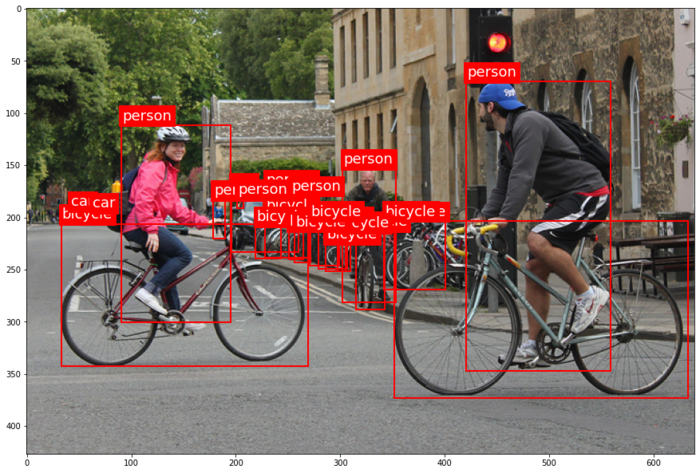
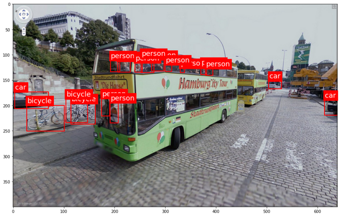
Below, you can find some samples from the training dataset. Each image contains multiple object annotations in the form of bounding boxes, denoted by their top-left corner coordinates (x, y) and their respective width and height (w, h). | |||
[[File:Img.png|700px]] [[File:Img2.png|700px]] | [[File:Img.png|700px]] [[File:Img2.png|700px]] | ||
====== | ====== YOLO model pipeline ====== | ||
'''Load the version YOLO network''' | |||
To begin the YOLO detection process, we need to load the YOLO network. YOLO, which stands for You Only Look Once, is an incredibly fast algorithm for multi-object detection that leverages a convolutional neural network (CNN) to identify and localize objects. | |||
In Python, I have created a pipeline for YOLO detection. To begin, we must download the pre-trained YOLO weight file and the YOLO configuration file. For this pipeline, I have chosen to use version v3 of YOLO. | |||
The YOLO neural network consists of 254 elements, including convolutional layers (conv), rectified linear units (relu), and other components. | |||
To load the YOLO model in Python, the following code snippet is used: | |||
net = cv.dnn.readNetFromDarknet('yolov3.cfg', 'yolov3.weights') | |||
'''Create a blob''' | |||
[[File:Blob from images header.png]] | |||
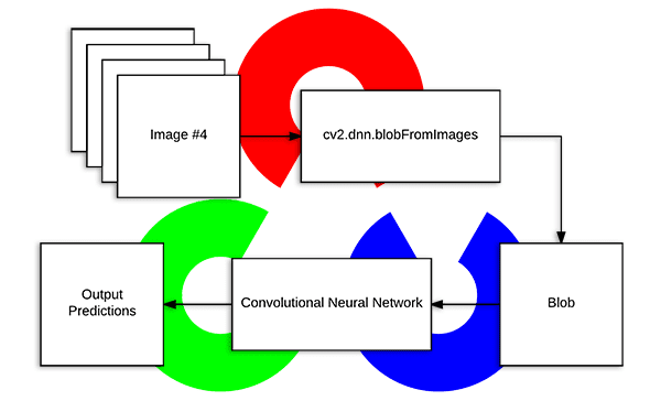
The input to the network is a | The input to the YOLO network is a blob object. To transform the image into a blob, we use the function '''cv.dnn.blobFromImage(img, scale, size, mean)'''. This step is crucial as it involves preprocessing the data to ensure accurate predictions from the deep neural network. | ||
The blobFromImage function performs the following operations: | |||
* '''Resizing''': It resizes the input image to a specific size required by the model. Deep learning models often have fixed input sizes, and the blobFromImage function ensures that the image is resized to match these requirements. | * '''Resizing''': It resizes the input image to a specific size required by the model. Deep learning models often have fixed input sizes, and the blobFromImage function ensures that the image is resized to match these requirements. | ||
| Line 152: | Line 189: | ||
* '''Channel Swapping''': It reorders the color channels of the image. Deep learning models often expect images in a specific channel order, such as RGB (Red, Green, Blue). If the input image has a different channel order, the blobFromImage function swaps the channels accordingly. | * '''Channel Swapping''': It reorders the color channels of the image. Deep learning models often expect images in a specific channel order, such as RGB (Red, Green, Blue). If the input image has a different channel order, the blobFromImage function swaps the channels accordingly. | ||
In this case, the scale factor is set to 1/255, which ensures that the lightness of the image remains the same as the original. | |||
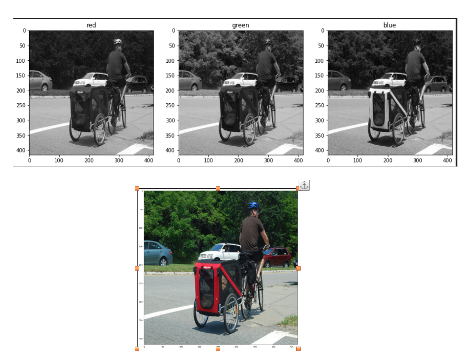
Once the image is transformed into a blob, it becomes a 4D NumPy array object with dimensions (images, channels, width, height) after resizing to (416, 416). The resulting blob consists of three channels: red, blue, and green. This can be visualized in the image below: | |||
[[File:1 255.png|Blob after preprocessing]] | |||
The blob object is then passed as input to the network, and the forward propagation is performed to retrieve all the layer names from the network and determine the output layers. The outputs object are vectors of length 85. | |||
[[File:OutputsYOLO.png]] | |||
* 4x the predicted bounding box (centerx, centery, width, height) | |||
* 1x box confidence: refers to the confidence score or probability assigned to the predicted bounding box. It represents the model's estimation of how confident it is that the bounding box accurately encloses an object in the image. | |||
* 80x class confidence : these scores indicate the probabilities or confidences that an object detected in the image belongs to a particular class among 80 classes | |||
'''Post processing ''' | |||
After obtaining the bounding boxes and their corresponding confidences from the output of an object detection model, it is common to apply a technique called Non-Maximum Suppression (NMS) to select the best bounding boxes. | |||
NMS is a post-processing step that helps eliminate redundant or overlapping bounding box detections. Its purpose is to select the most accurate and representative bounding boxes while removing duplicates or highly overlapping detections. | |||
In OpenCV, the cv.dnn.NMSBoxes() function is a convenient utility function that performs NMS. It accepts several parameters to fine-tune its behavior: | |||
* '''boxes''': This parameter represents the bounding boxes detected in the image. Each bounding box is typically represented as a list of four values (x, y, width, height) or as a tuple. | |||
* '''confidences''': This parameter contains the confidence scores associated with each bounding box. The confidence scores indicate the likelihood that the corresponding bounding box contains an object of interest. | |||
*'''score_threshold''': This parameter specifies the minimum confidence score threshold for considering a bounding box during NMS. Any bounding box with a confidence score below this threshold will be disregarded. | |||
*'''nms_threshold''': This parameter determines the overlap threshold for suppressing redundant bounding boxes. If the overlap between two bounding boxes exceeds this threshold, the one with the lower confidence score is suppressed. | |||
The '''cv.dnn.NMSBoxes()''' function returns the indices of the selected bounding boxes that passed the NMS process. These indices correspond to the original list of bounding boxes and confidences, allowing you to access the selected boxes and their associated information. | |||
====== Brainstorming: Multiple Options for Object Tagging in DigiKam ====== | |||
In this project, my goal is to empower users with the ability to choose specific options from a predefined set of 80 classes for automatic tagging in input images within DigiKam. We achieve this by leveraging the object detection capabilities of YOLO. | |||
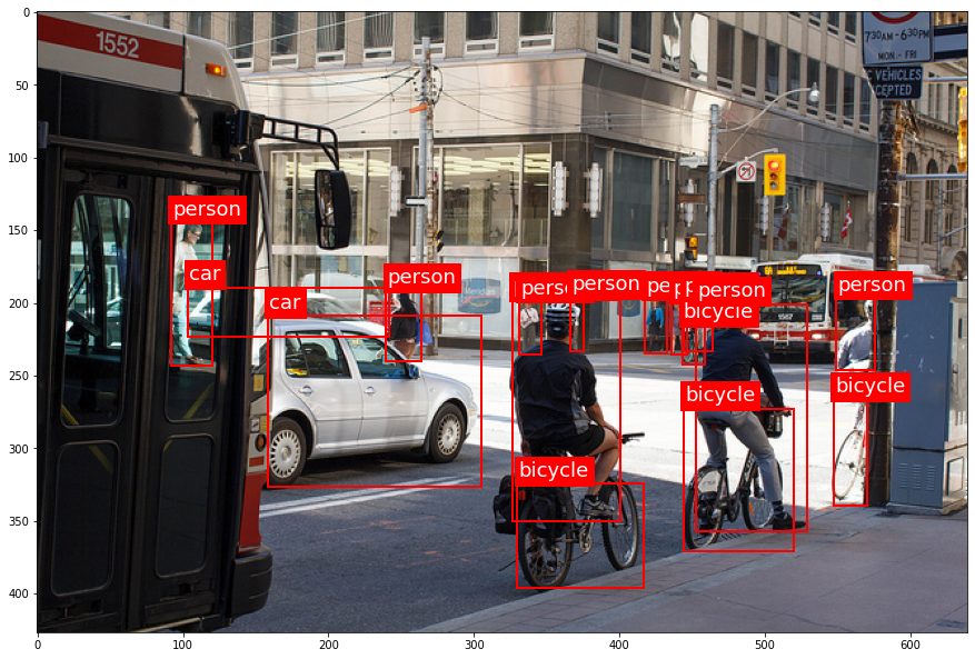
Let's take a look at an example from my research notebook, this picture include some objects like 'person', 'bike', 'car', 'bus': | |||
[[File:Ex1.png]] | |||
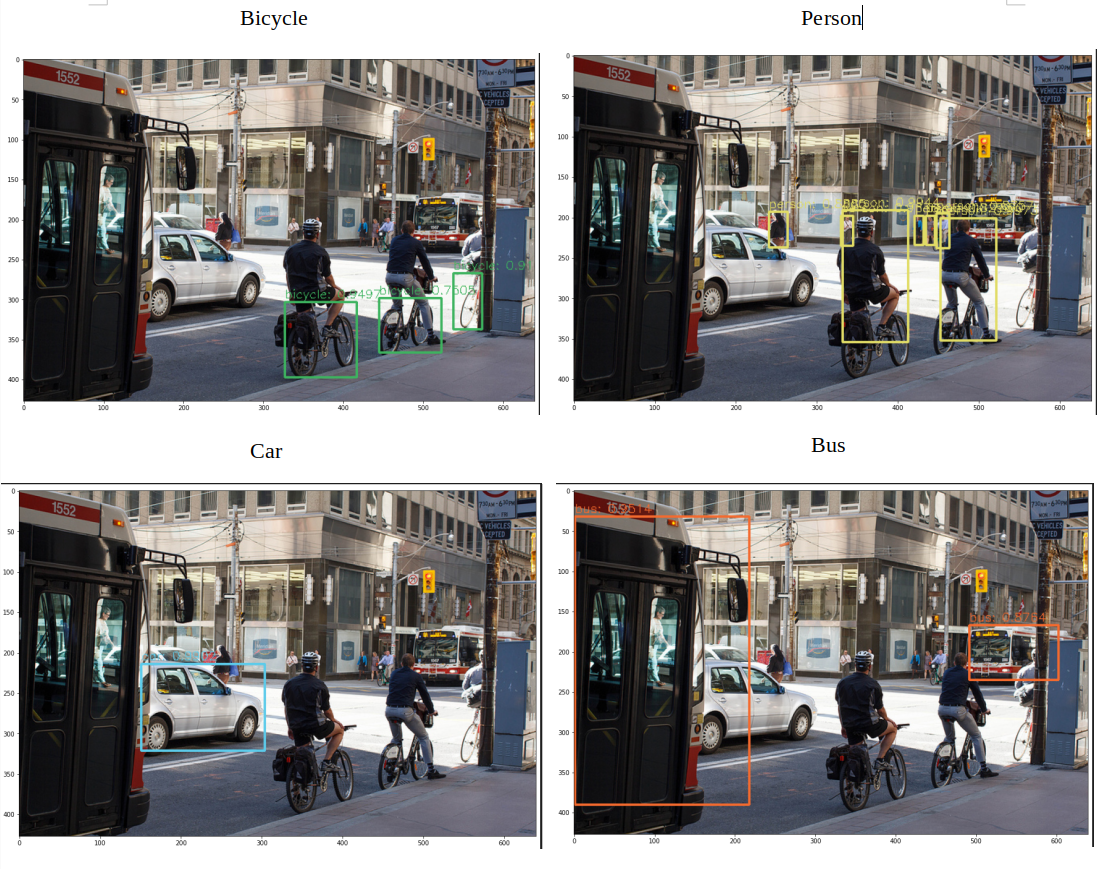
After applying the YOLO model to the image, we obtain the following visualization with separated option from user: | |||
[[File:Object detection img.png]] | |||
Each image in the visualization represents a detected object, accompanied by a bounding box that highlights its location. This provides users with a clear understanding of the detected objects in the image. | |||
In DigiKam, users have the freedom to select specific objects from the detected classes and assign appropriate tags to them. This flexibility allows for a personalized approach to organizing and categorizing images based on individual preferences and requirements. | |||
===== (Week 3 - 4) ===== | ===== (Week 3 - 4) ===== | ||
'''DONE''' | |||
* Researched and created the Deeplearning pipeline to bencmark the different yolo version in term of the accuracy and inference time, decided which one should be intergrated into digiKam. | |||
* Exported ONNX file for yoloVersion for the inference. | |||
* Documentation | |||
'''TODO''' | |||
* Develop a mock widget in C++ | |||
====== YOLOv3 and YOLOv4 Performance ====== | |||
Currently, In face engine, '''digiKam''' is using Yolov3 and SSD for recognition, the accuracy is better considering Yolov3. As a rough estimate, on a modern CPU, YOLOv3 can achieve around 1-2 FPS with an inference time of 500-1000 milliseconds per image. | |||
About object detection project, I actually benchmark this term for yolov3 and yolov4 in my local machine ('''cpu amd ryzen 5 5600h with radeon graphics with 6 cores'''), for running through out 45 validation images dataset, in order to calculate the average inferebnce time and FPS (frames per second) of the YOLOv3 and v4. And I can see the inference time was the same as the estimate. | |||
Provide the like of notebook here: | |||
{| class="wikitable" | |||
|+ Inference times and FPS YOLOv3 and YOLOv4 in CPU | |||
|- | |||
! YOLO version !! Average Inference Times !! Average FPS | |||
|- | |||
| YOLOV3 || 673.43 ms|| 1.5 frames/s | |||
|- | |||
| YOLOV4|| 772 ms|| 1.3 frames/s | |||
|} | |||
It appears that YOLOv3 performs slightly better than YOLOv4 in terms of both inference time and FPS. YOLOv3 has a lower average inference time and a higher average FPS, indicating faster processing and better real-time performance compared to YOLOv4 on the tested CPU. YOLOv4 is generally considered to be a more advanced and complex model compared to YOLOv3. It introduces several architectural changes and additional components to improve accuracy and detection capabilities. However, these advancements may come at the cost of increased computational requirements, resulting in longer inference times and lower FPS. | |||
====== Selection model (Experiences with YOLOv5) --- Convert YOLO model to ONNX format ====== | |||
In order to address this issue, several questions should be taken into consideration when selecting a model: | |||
* Which YOLO model is the fastest on the CPU? | |||
* Which YOLO model is the most accurate? | |||
'''Load YOLOV5 model using onnx:''' | |||
Since YOLOv5 is implemented in PyTorch rather than the Darknet framework, we cannot directly use the cv2.dnn.readNetFromDarknet() function in OpenCV to load the YOLOv5 model. Currently in face detection in digiKam, we used the readNetFromDarknet() function which is specifically used to load models that are trained using the Darknet framework. | |||
Instead, we need to convert the YOLOv5 model to the ONNX format and then use the cv2.dnn.readNetFromONNX() function in OpenCV to load the ONNX model. In fact, ONNX stands for Open Neural Network Exchange. It is an open-source format designed for interoperability between different deep learning frameworks. ONNX allows to export trained models from one framework and import them into another, making it easier to deploy and use models across various platforms and frameworks. Luckyly, OpenCV provides a familiar and easy-to-use API for loading, running, and post-processing ONNX models. It allows me to integrate ONNX models seamlessly into our computer vision pipelines. | |||
cv2.dnn.readNetFromONNX('yolov5nano.onnx') | |||
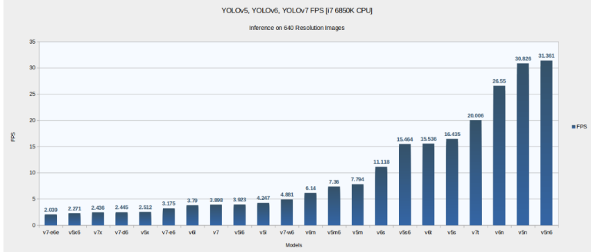
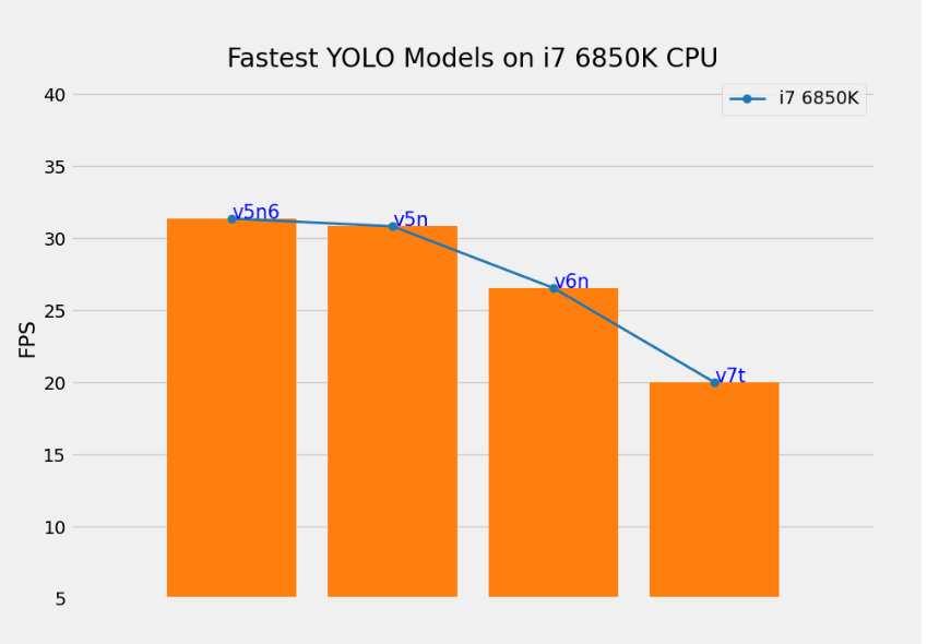
Although the numbers vary depending on the CPU architecture, we can find a similar trend for the speed. The smaller the model, the faster it is on the CPU. Considering the following research in [https://learnopencv.com/performance-comparison-of-yolo-models/#FPS-Performance-Comparison-of-YOLO-Models-on-CPU this aricle] we find that YOLOv5 Nano and Nano P6 models are the fastest results on 640 resolution images and 1280 resolution image. | |||
[[File:YOLOv5 v6 v7 CPU.png]] | |||
[[File:V5 v6 v7 i7 6850K CPU.png]] | |||
However in term of accuracy, we need to consider the larger models from each family (v5x, v6l, v7x) perform quite well. Because, I intend to use COCO classes for tag assigments, so then using one of the mentioned pre-trained models will give you very accurate predictions. | |||
Looking at the figure below from the [https://learnopencv.com/performance-comparison-of-yolo-models/#FPS-Performance-Comparison-of-YOLO-Models-on-CPU article] | |||
{| class="wikitable" | |||
|+ Inference times and FPS YOLOv3 and YOLOv4 in CPU | |||
|- | |||
! YOLO version !! Average Inference Times !! Average FPS | |||
|- | |||
| YOLOV3 || 673.43 ms|| 1.5 frames/s | |||
|- | |||
| YOLOV4 || 772.6 ms|| 1.3 frames/s | |||
|- | |||
| YOLOV5 nano || 80 ms || 14 frames/s | |||
|- | |||
| YOLOV5 Xlarge || 1442 ms|| 1.3 frames/s | |||
|} | |||
Some remarks I would like to discuss: | |||
YOLOv5 Nano: YOLOv5 Nano demonstrates significantly faster inference times and higher FPS compared to YOLOv3 and YOLOv4. It has an average inference time of 80 ms, resulting in 14 frames per second. YOLOv5 Nano's lightweight design makes it well-suited for low-power or resource-constrained devices where real-time object detection is desired. | |||
YOLOv5 XLarge has a relatively longer inference time of 1442 ms, resulting in 1.3 frames per second. While it offers potentially higher accuracy due to its larger model size, it sacrifices real-time performance. YOLOv5 XLarge might be more suitable for scenarios where accuracy is prioritized over speed. | |||
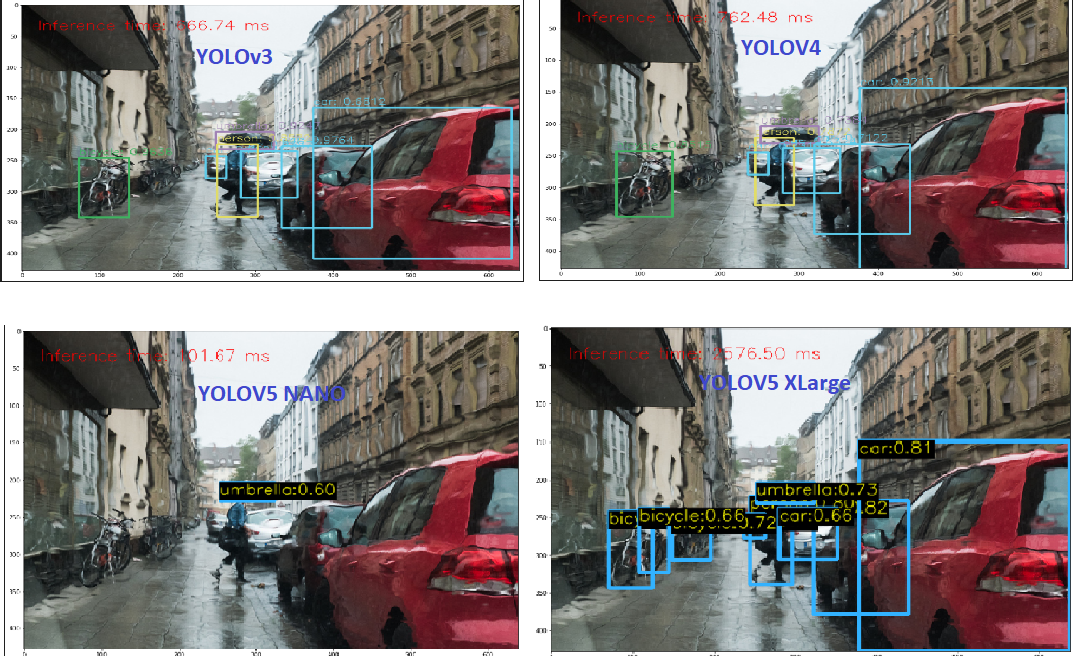
Yolo familly detect quite good mostly in many kind of images. The following results can release the good output with 80 pretrained-objects. Regarding the observation about YOLOv5 Nano performing well in blurred or complex images, it's worth noting that the model's performance can vary based on factors like dataset, training methodology, and specific use cases. YOLOv5 models, in general, offer a trade-off between accuracy and speed, with larger models providing higher accuracy at the cost of slower inference times . The image below shows a comparison of object detection with these familly of YOLOversion. | |||
[[File:Yolov345.png]] | |||
Precision measures the accuracy of positive predictions, while recall measures the completeness of positive predictions. High precision and high recall are desirable. In the case of the YOLO algorithm, it tends to predict correct examples with a relatively higher precision score. However, it may not detect all the desired objects, impacting its recall. When considering the different YOLO models, YOLO X Large stands out by achieving very high precision and recall scores. This model outperforms the others and is capable of detecting even smaller objects accurately. | |||
In conclusion, next pharse: | |||
* I plan to develop a testing mock GUI in C++ to benchmark various algorithms before integrating them into digiKam tools. This GUI will specifically focus on benchmarking the latest version of YOLO for object detection. It will provide support for benchmarking multiple versions of object detection algorithms, displaying frames per second (FPS), and measuring inference times. | |||
* Additionally, it is important to consider hardware acceleration in this use case. OpenCV offers optimizations for hardware acceleration, such as leveraging specialized libraries like OpenVINO or utilizing GPU acceleration. These optimizations can significantly enhance the performance of running ONNX models on compatible hardware. | |||
===== (Week 5 - 6) ===== | ===== (Week 5 - 6) ===== | ||
'''DONE''' : | |||
* Create Integration testing tools to benchmark dnn model detector. | |||
* Documentation. | |||
'''Main merger request''': | |||
https://invent.kde.org/graphics/digikam/-/merge_requests/221 | |||
'''TODO''' : | |||
* Etude the code base to integrate auto-tags features into yhe Maintenance or BQM tools. | |||
* Focus on applying the detector in batch | |||
* Documentation. | |||
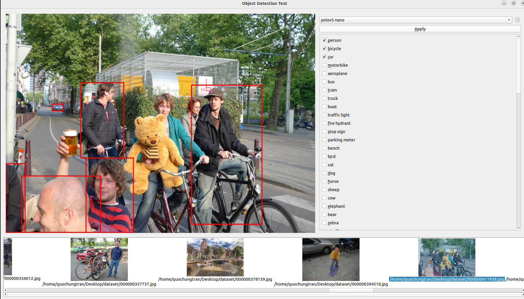
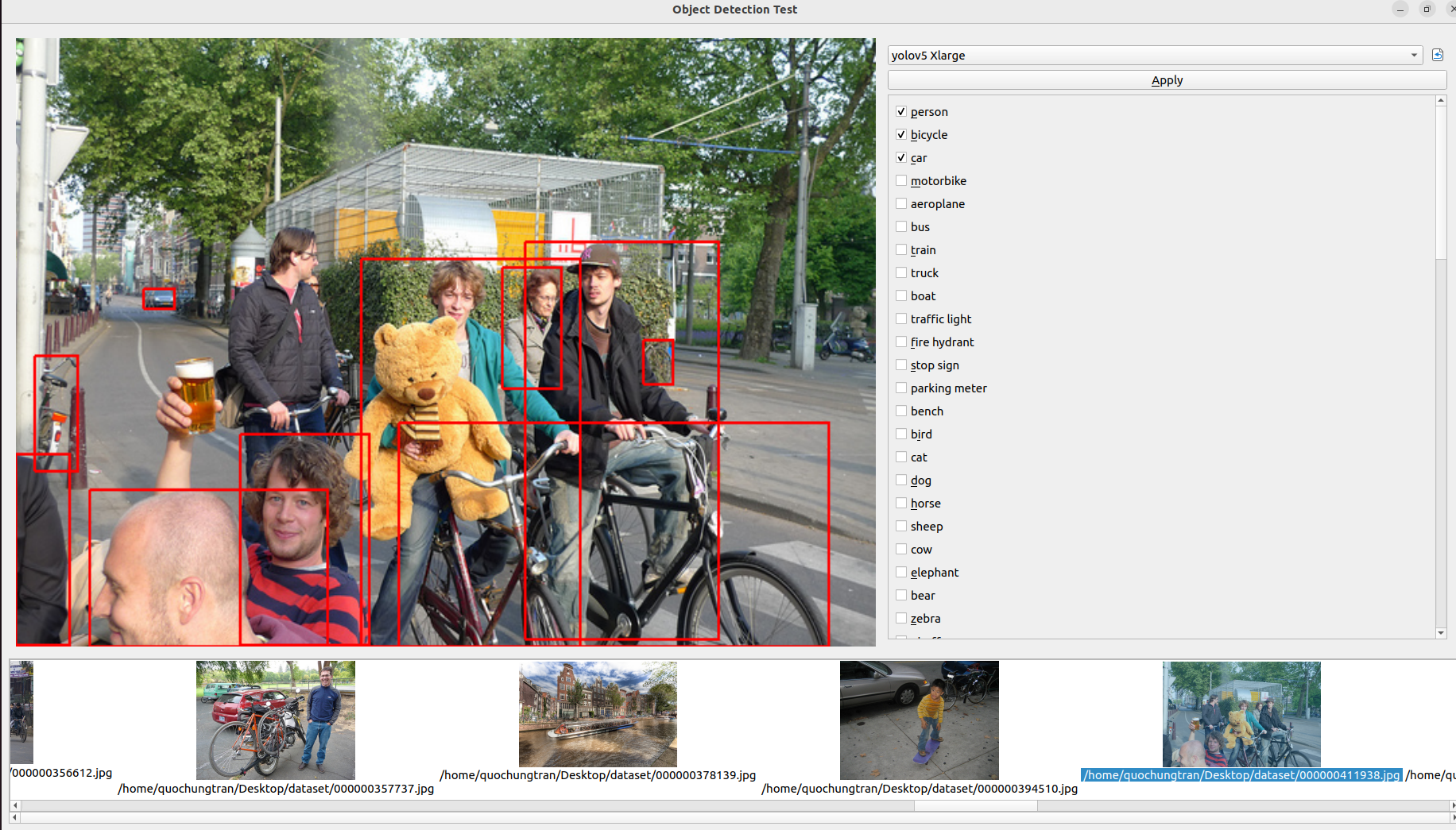
After several week of researchs, I decided to choose 2 model YOLOv5nano and YOLOv5 XLarge to deploy into digiKam. First of all, I create an integration testing tools. Integration testing plays a crucial role in ensuring the seamless functioning of software systems. As part of my ongoing efforts to optimize testing processes, I am excited to announce my plan to create a Merge Request (MR) for integrating benchmarking tools with the popular YOLO (You Only Look Once) version. This MR aims to enhance the capabilities of the testing suite by introducing two essential components: a user-friendly control panel and an intuitive image area for displaying detected objects. In this blog post, I will outline the features of these tools and highlight their superior performance compared to existing Python-based solutions. | |||
The integration testing tools I'm developing will consist of two primary elements: | |||
* Control Panel with Model Selection and Predefined Classes: | |||
The control panel will serve as the central interface for the benchmarking process. It will provide users with a range of options to select the desired YOLO model for evaluation. Additionally, the control panel will feature a comprehensive library of 80 predefined classes, enabling efficient testing across a wide range of object detection scenarios, selecting by users. | |||
* Image Area for Displaying Detected Objects: | |||
To provide a visually engaging and informative experience, the tools will incorporate an image area that displays all the detected objects. This intuitive interface allows users to observe the precision and accuracy of the YOLO models in action. By visualizing the results, testers can gain valuable insights into the performance and reliability of the integration tests. | |||
Unparalleled Performance: | |||
One of the primary reasons for integrating these benchmarking tools into your testing suite is their exceptional performance. In terms of inference time per image, the tools outperform existing Python-based alternatives. Let's take a look at the average performance of the two YOLO models when running on a CPU: | |||
*'''YOLOv5 Nano''': With an impressive average inference time of just 57 ms (compared to 80ms in Python), the YOLOv5 Nano model offers exceptional speed and efficiency. It enables you to swiftly evaluate the integration of smaller-scale object detection scenarios. | |||
*'''YOLOv5 XLarge''': For more complex object detection requirements, the YOLOv5 XLarge model showcases remarkable capabilities. Despite the additional complexity, it still maintains an average inference time of 724 milliseconds (compared to 1400ms in Python), ensuring reliable and precise testing for larger-scale scenarios. | |||
[[File:TestModel.webm]] | |||
[[File:Test gui1.png]] | |||
[[File:Test gui2.png]] | |||
===== (Week 7 - 8) ===== | ===== (Week 7 - 8) ===== | ||
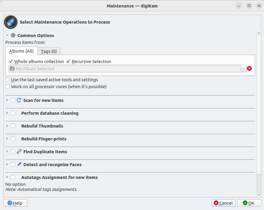
In this week, I tried to study how to integrate the feature into Maintenance and BQM tools, show let me introduce some short information about these tools. | |||
Following Gilles's propositions: | |||
* Look how Quality sorting, the tool (eg the Maintenance or BQM tools) will not ask to the user if the estimated values (Pick Labels) are fine or no while the analysis. There are settings to route the values at the right place in the database, all is done automatically. Adding a new maintenance tool for autotagging feature in the chained process (Maintenance are not yet a plugin). | |||
Maintenance is a tool running processes in the background to maintain image collections and database contents. The list of tools is presented in a sequential order and cannot be changed. Only the tools to activate or deactivate during a maintenance session can be selected. The sequence of tools is relevant of the order to populate the information in database on the first time, and the way to use these information in a second time. So the mission here is add the new checkbox widget for auto tags process int the existing maintenance dialog (showed in the image below): | |||
[[File:Mtn1.png]] | |||
One of the tools available from the list are listed below using deep learning is: '''Detect and Recognize Faces''': perform automatic faces management updates and '''Image Quality Sorter:''' perform an automatic scan of items to sort items by quality and apply Pick Labels in database. This is mostly the core engine and the GUI described in this documentation : | |||
https://docs.digikam.org/en/batch_queue.html | |||
* Adding a new BQM tool (in this case it's a plugin). | |||
DigiKam features a batch queue manager in a separate window to easily process in batch items, aka filtering, converting, transforming, etc. It works with all supported image formats including RAW files. | |||
* Adding a new menu entry to process item from preview mode (typically to parse one item current visualized by end-user). | |||
In this case we can follow the structure as People preview mode for Face recognition. | |||
===== (Week 9 - 10) ===== | ===== (Week 9 - 10) ===== | ||
'''DONE''' : | |||
* Developed a checkbox widget for autotag assignments within the Digikam Maintenance dialog. | |||
* Established a connection between the frontend widget and backend to enable tag generation during the Maintenance process in Digikam. | |||
* Documentation. | |||
'''TODO''' : | |||
* Using API from ItemInfo object to populate tags automatically in database (create new TagAlbum accordingly). | |||
* Etude more lightweight model. | |||
====== Architecture of Maintenance Tool ====== | |||
'''Main Commits''' : | |||
[https://invent.kde.org/graphics/digikam/-/merge_requests/221/diffs?commit_id=606bcd54784983c8a2fb1ad1e4c122575770a527 606bcd54] | |||
[https://invent.kde.org/graphics/digikam/-/merge%20requests/221/diffs?commit%20id=078b8a98bf626d5c1bcfd393e2f42b8b801edf1e 078b8a98] | |||
[https://invent.kde.org/graphics/digikam/-/merge_requests/221/diffs?commit_id=5588e928e49d8f74e3f9ece82d9c6fae33d5724a 5588e928] | |||
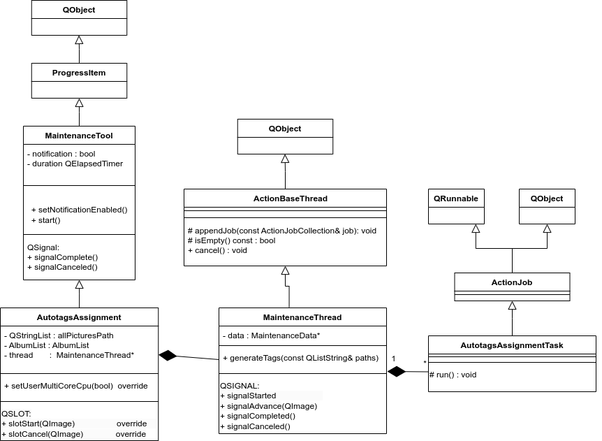
This process will use an internal Maintenance multi-thread for generate tags automatically from input images. Classes in this part will be implemented based on existing objects to manage and chain threads in digikam. The idea is inspired by using '''QThreadPool''' and '''QRunnable'''. Existing threads can be reused for new tasks, and '''QThreadPool''' is a collection of reusable QThreads. The part '''MaintenanceThread''' manages the functioning of '''AutotagsAssignmentTask'''. Concretely, MaintenanceThread manages the instantiations of AutotagsAssignmentTask. Each AutotagsAssignmentTask will initialize one AutoTags engine object to manage one URL of an image. | |||
The purpose is to allow each process to run in parallel and stop properly. The '''run()''' method of object AutotagsAssignmentTask is a virtual method that will be reimplemented to facilitate advanced thread management. Here is the architecture of this part: | |||
[[File:UML mtntools.png]] | |||
'''MaintenanceThread''' is encapsulated by '''AutotagsAssignment''' which is a MaintenanceTool widget object generatively used around the code base, applied for another Maintenance processes. | |||
====== Main back-end AutoTagging feature ====== | |||
'''Main Commits''' : | |||
[https://invent.kde.org/graphics/digikam/-/merge_requests/221/diffs?commit_id=606bcd54784983c8a2fb1ad1e4c122575770a527 606bcd54] | |||
As per my mentors' suggestion, the utilization of item keywords (tags) usually suffices to populate information derived from AI analysis, aimed at identifying forms, objects, locations, flora, fauna, and more. The API for this purpose already exists within the existing database, facilitating the integration of such information. Therefore, in this context, the predicted classes hold greater significance. | |||
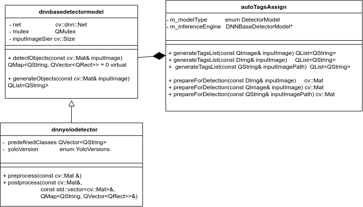
I implement a class named "AutoTags" for this purpose. This class is designed to initialize the relevant model, preprocess the input image for detection, and subsequently generate and store tags based on the output classes, which are then released as the final results. | |||
[[File:UMLtagBackend.png]] | |||
In this case, I used '''the Factory Pattern''' which is a creational design pattern in software engineering. It is used to create objects without specifying the exact class of object that will be created. Instead of calling a constructor directly to create an object, the Factory Pattern uses a separate factory class or method to handle object creation. | |||
The main idea behind the Factory Pattern is to encapsulate the Deeplearning creation process and provide a way to create objects based on certain conditions or parameters (the type of different models). This can help improve code organization, maintainability, and flexibility, particularly in scenarios where a multitude of subcategories (Deep Learning models) exist or diverse implementations of a class are required (as observed in tasks like deploying inference models and executing operations). | |||
===== (Week 11 - 12) ===== | ===== (Week 11 - 12) ===== | ||
In these weeks, I focus on implement in : | |||
- Bench marking model for inference in batch images (it means that feed forward in multiple images in the same times rather than a single image). | |||
- Implemented settings widget in maintenance tools. | |||
'''Main Commits''' : | |||
[https://invent.kde.org/graphics/digikam/-/merge_requests/221/diffs?commit_id=d38d3508e8a5a4b6e66ffe492718be3da3b746b3 d38d3508] | |||
====== Implemented Auto tagging process ====== | |||
So in these weeks, I experimented running the inference in batch. In fact, in the realm of deep learning, '''batch processing''' is a pivotal technique that enables the concurrent processing of multiple input data points or images, rather than handling them one by one in a sequential loop. I would like benchmark the performance of the models in CPU to see the if it work well in this specified hardware. | |||
To harness the potential of batch processing effectively, it's essential to convert our deep learning model into the ONNX (Open Neural Network Exchange) format. For the YOLO, I have used the piece of codes (pipeline [https://colab.research.google.com/github/spmallick/learnopencv/blob/master/Object-Detection-using-YOLOv5-and-OpenCV-DNN-in-CPP-and-Python/Convert_PyTorch_models.ipynb#scrollTo=ITUKhgc2P4T6 pipeline_to_convert_onnx]) from ggcolab for converting the model to ONNX file | |||
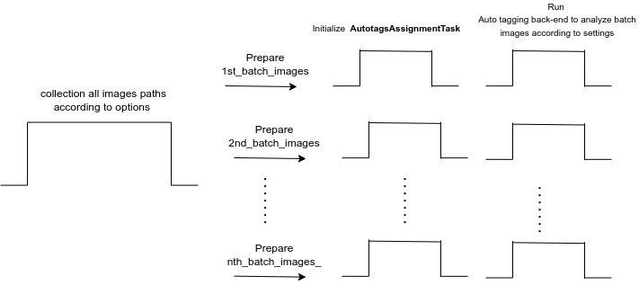
So inside of the digikam code, The pipeline is initialized in the following images : | |||
[[File:Auto tag process.drawio.png]] | |||
so firstly, The autotags process will collect all picture data paths to be ready for the started stage, according to the options whether users want to assigned the non-assigned items or not. And then, the internal thread will handle auto-tagging processing images, each batch images will be in charged with a job (AutotaggingTask Objects), the number of job is equivalent of the number of batch images paths (defaulted 1) : | |||
Num_of_jobs = Size_of_album / batch_size | |||
====== New pre-trained model for images classification ====== | |||
Because it's related to image classification. So I wanted to implement pre-trained model ResNet which is a specific variant of the Residual Network (ResNet) architecture designed for solving image classification problems. It's a deep convolutional neural network (CNN) architecture that has demonstrated outstanding performance on image classification tasks. This variety helps users have more choices when using this model for objects auto tagging. | |||
Objects names of ImageNet : https://deeplearning.cms.waikato.ac.nz/user-guide/class-maps/IMAGENET/ | |||
====== The performance between different batch sizes ====== | |||
I measured the performance of each models for different of batch images in CPU harware with the same input images '''(320 x 320)''', showing in the following dashboard: | |||
{| class="wikitable" | |||
|+ Performance of each model for different of batch_size images | |||
|- | |||
! Model !! Batch size !! Inference (net 's forward process) !! FPS ((1000/(Inference_time / batch_size)) !! Latency of the whole process (include pre and post processes) | |||
|- | |||
| YOLOv5 Nano || 1 || 19ms || 53 frames/s || 40ms / frame | |||
|- | |||
| YOLOv5 Nano || 10 || 215ms (21.5ms/frame) || 46,5 frames/s || 358ms (35,8ms/frame) | |||
|- | |||
| YOLOv5 Nano || 16 || 389ms (24.3ms/frame) || 41 frames/s || 552ms (34ms/frame) | |||
|- | |||
| YOLOv5 XLarge || 1 || 200ms || 5 frames/s || 775 ms / frame | |||
|- | |||
| YOLOv5 XLarge || 10 || 2888(288ms/frame) || 4 frames/s || 4049ms (405ms/frame) | |||
|- | |||
| YOLOv5 XLarge || 16 || 4944(309ms/frame) || 3 frames/s || 6267ms(391ms/frame) | |||
|- | |||
| RESNET50 || 1 || 37ms || 27 frames/s || 200ms / frame | |||
|} | |||
Based on these experiences, it's evident that running inference with a batch size greater than 1 on the CPU results in slower inference times compared to using a batch size of 1. However, this approach can offer significant advantages for the overall process, particularly during post-processing. When we create a buffer and extract objects or initialize objects, run the inference multiple times can introduce the risk of slowing down the entire process. Additionally, it's worth noting that integrating with a '''GPU''' can further enhance inference times | |||
NOTE : If we are developing an application that needs to run on multiple types of hardware, then OpenCL may be the better choice. However, if we are developing an application that will only run on NVIDIA GPUs, then CUDA may be the simpler option. | |||
So in this section, we would like to use OpenCl for GPU computation. | |||
So I decided to add an option in selecting models (3 models above) with batch size 16. | |||
===== (Week 13 - 14 - 15- 16) ===== | |||
To-Do | |||
- Study the Face Engine Pipeline | |||
===== Feature maintenance settings ===== | |||
I have implemented dedicated maintenance settings for our auto-tagging features. These settings provide the flexibility to: | |||
1. Rescan the entire folder or scan items with unassigned tags. | |||
2. Select a model from the following options: | |||
'''YOLOV5 Nano''': This is the fastest model for labeling images. | |||
'''YOLOv5 Xlarge''': An updated version of YOLOv5, known for its enhanced accuracy, ideal for users who need precise tagging for a smaller number of images. | |||
'''Resnet''': Designed for classifying more than 1000 different objects, offering a broader range of labeling options. | |||
These settings are accessible through the Maintenance Settings object, which contains all the optional configurations within the Maintenance Tools. | |||
The user interface for these settings can be seen in the following images: | |||
[[File:Screenshot from 2023-10-20 17-27-37.png]] | |||
Additionally, you can watch a screencast showcasing the process of generating tags in Digikam's Maintenance Tool: | |||
[[File:Screencast from 20-10-2023 17-23-36.webm]] | |||
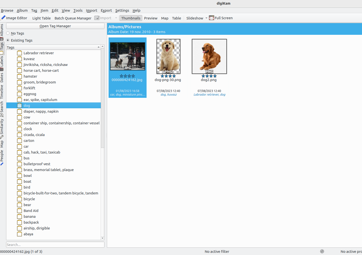
All the tag is showed in the screen : | |||
[[File:Screenshot from 2023-10-20 17-57-21.png]] | |||
===== Conculsion ===== | |||
During the significant coding period of GSoC 2023, we implemented the tool to auto tagging the image. It's still have some couple of problems as the hardware issue to handle out but the main ideas have been populated. Now I switch into studying the face engineer, an feature to face tagging automatically. | |||
At the end of this project, the following bugs are supposed to be fixed: | |||
https://bugs.kde.org/show_bug.cgi?id=440582 | |||
https://bugs.kde.org/show_bug.cgi?id=416988 | |||
==== (Week 17 - 18 - 19 - 20) ==== | |||
In recent weeks, I have been dedicated to addressing the challenges faced by the engine and have thoroughly examined the code base. Subsequently, I formulate a plan to identify the key components that require our attention. | |||
===== Identifying the Issue ===== | |||
In our Bugzilla reports, we have identified the following problems: | |||
Bugzilla: | |||
* Face recognition, see and edit references: https://bugs.kde.org/show_bug.cgi?id=471183 | |||
* Face recognition malfunction: https://bugs.kde.org/show_bug.cgi?id=429230 | |||
* Face detection is extremely slow - face recognition is almost impossible : https://bugs.kde.org/show_bug.cgi?id=464266 | |||
These issues stem from the reports mentioned above: | |||
One of the primary concerns is the sluggish performance of image detection using SSD and Yolov3, especially when processing a large volume of images. This delay is a major setback. | |||
The core issue lies in the accuracy of recognition. Blurred images are often falsely recognized as faces, and there are instances where unexpected images are misidentified as individuals. Furthermore, even after users scan the images folder, these unexpected detections persist. In essence, the detection process undergoes re-scanning, and the erroneous results remain associated with the 'unknown' tag. These anomalies can be considered as noise that interferes with the recognition process. | |||
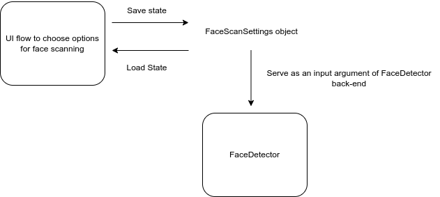
For the maintainability and improvement for the future, and because of the complexity, I will document the current UI flow and back-end flow. The connection between the UI and backend is throughout a class we call '''FaceScanSettings'''. | |||
[[File:DIAGRAM-Trang-4.drawio.png]] | |||
===== Face Engine UI Flow ===== | |||
These components collectively make up the user interface and settings for the face scanning widget. Users can configure the scanning workflow, select albums, and adjust various settings related to accuracy, models, and CPU usage through this widget. | |||
These settings of the widget will be stored as the attributes in the '''FaceScanSettings''' object. This class defines settings related to face scanning in the digiKam project and could be used to send the information from the UI . The components of this class are as follows: | |||
Workflow settings | |||
* ScanTask task: An instance of the ScanTask enumeration representing the selected scanning task (Detect or recognize jobs). | |||
* AlreadyScannedHandling alreadyScannedHandling: An instance of the AlreadyScannedHandling enumeration representing how already scanned faces should be handled. | |||
Selecting the proper folder for training | |||
* bool wholeAlbums: A boolean indicating whether whole albums are checked for scanning. | |||
* AlbumList albums: A list of albums to scan. This may include physical or virtual albums. | |||
* ItemInfoList infos: A list of image information to scan. | |||
Model Settings | |||
* bool useFullCpu: A boolean indicating whether the full CPU processing power should be used for scanning. | |||
* bool useYoloV3: A boolean indicating whether the Yolo V3 model should be used for scanning. | |||
* double accuracy: A double representing the detection accuracy. | |||
===== Current Face management (Back-end) ===== | |||
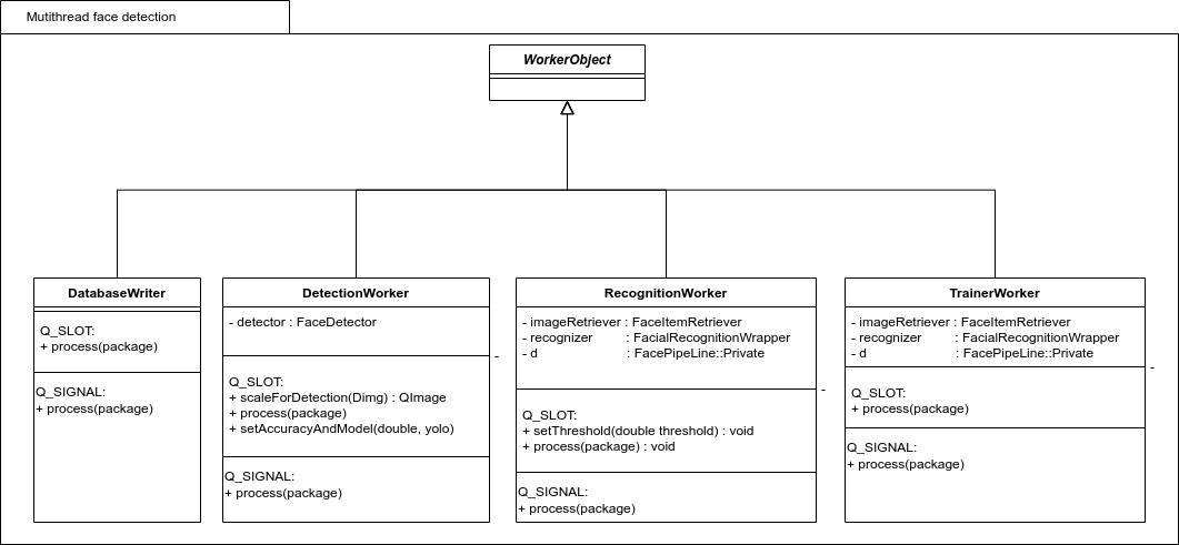
There are workers which play integrated, multi thread face detection/ recognition roles. It's inherited from a common object | |||
'''WorkerObject''', which is the WorkerObject class is a part of the digiKam project and provides a framework for multithreaded processing. It allows you to execute slots in a separate thread and manage the state and deactivation of the worker object. It provides methods for scheduling, deactivation, and thread priority management. It emits signals to indicate when work begins and ends. The class uses the Qt framework for multithreading and event handling. | |||
The class provides various public methods, including: | |||
'''state()''': Returns the current state of the worker object. | |||
'''wait()''': Blocks the calling thread until the worker object finishes. | |||
'''setPriority(QThread::Priority priority)''': Sets the thread priority. | |||
'''priority()''': Returns the current thread priority. | |||
'''connectAndSchedule()''': Helper methods for connecting signals and scheduling the worker object. | |||
'''schedule()''': Starts the execution of the worker object. | |||
'''deactivate(DeactivatingMode mode)''': Quits the execution of the worker object. | |||
and the most core function is process(const FacePipelineExtendedPackage::Ptr& package) is used to run the Face detector and recognized backend to handle the arrived in one package (not in batch), and emits the signal when it's done, and do the next the process in the pipeline. | |||
[[File:Thread recognization.png]] | |||
'''Current face Pipeline:''' | |||
Class FacePipeline is used for managing the face detection and recognition pipeline in the digiKam project. It allows you to configure and plug in various components to process images, and it provides methods for training, confirming, and editing facial recognition results. | |||
Some important components in FacePipeline: | |||
- The '''construct()''' function in the code you provided is responsible for setting up the face detection and recognition pipeline. It connects various components, such as image loaders, detectors, recognizer, database writers, and trainers, in the specified order to process images. The function may also set the thread priority for the processing threads. You can control the priority of threads used for different components to manage system resource usage. | |||
Returning the Constructed Pipeline. Once the connections are established, the pipeline is ready for processing. The pipeline consists of a sequence of components connected by signals and slots. | |||
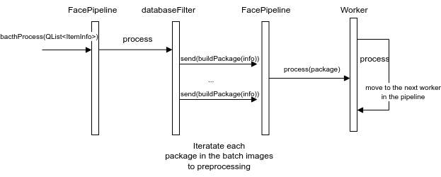
- The function '''bacthProcess(QListInfo)''' encapsulate the running the low level of each worker we discussed above. You can see the the schema | |||
[[File:Pipeline.drawio.png]] | |||
The comment lists the key components that can be added to the pipeline. Each component serves a specific purpose in the face detection and recognition process: | |||
* Database Filter: This component prepares database records and can filter out items based on certain criteria. The filter mode is specified using FilterMode. | |||
* Preview Loader: If a preview loader is not plugged in, you must provide a DImg (an image) for face detection and recognition. The preview loader may be responsible for loading these images. | |||
* Face Detector: This component detects faces in the provided images. If no recognizer is plugged, all detected faces are marked as "the unknown person." | |||
* Face Recognizer: If no detector is plugged, this component processes only already scanned faces marked as unknown. These faces are implicitly read from the database. | |||
* DatabaseWriter: This component writes the detection and recognition results to the database. It doesn't affect the trainer, which works on a different storage. | |||
* DatabaseEditor: This component can be used to confirm or reject faces in the database. | |||
The comment mentions a '''PlugParallel''' method, which seems to be an alternative way to plug components into the pipeline. It suggests that, depending on the number of processor cores and memory availability, more than one element may be plugged and processed in parallel. This can potentially speed up the processing. | |||
Supported Combinations: | |||
The comment provides examples of supported combinations of components in the pipeline. These combinations show how different components can be connected to create a functional processing pipeline. The notation (Component A ->) indicates that Component A is plugged into the pipeline, and the arrow points to the next component in the sequence. The combinations include: | |||
(Database Filter ->) (Preview Loader ->) Detector -> Recognizer (-> DatabaseWriter) | |||
(Database Filter ->) (Preview Loader ->) Detector (-> DatabaseWriter) | |||
(Database Filter ->) (Preview Loader ->) Recognizer (-> DatabaseWriter) | |||
DatabaseEditor | |||
===== Brainstorming ===== | |||
The logic of the detector still relies on YOLOv3 and SSD for processing one image at a time, rather than in batch mode, which involves matrix multiplication. Repeated initialization of the model can result in time wastage. | |||
In terms of model accuracy, as per Nghia's GSOC report, the recent update to the face recognition engine has substantially improved accuracy, and has successfully integrated the Facenet DNN model into the face engines. This new update increases the accuracy of facial recognition to 98.54%, but it also increases 4 times the size of the face embedding to be stored. T-SNE data projection is integrated into the recognition process. It reduces the dimension of face embedding from 512 to 2, which improves accuracy and reduces processing time. In general, t-SNE takes 12ms/face and recognition takes less than 1ms/face. | |||
However, the repetition of face embedding extraction, especially with the addition of T-SNE data projection, consumes a significant amount of time. One straightforward solution to avoid this redundancy is to compute and save the face embedding immediately after a face is detected, making it available for future use. | |||
Introducing face embedding extraction into the detection pipeline may potentially extend the processing time. | |||
* In Nghia's words, the synchronous processing mechanism results in unnecessary waiting time and blocks the main thread of the application. As a solution, we have decided to transition the processing mechanism in face pipelines to an asynchronous mode. This means that data can be queued in a worker at one point and processed at another time. | |||
* We could explore the use of more modern models to enhance accuracy, and additionally, leverage batch inference. This entails initializing the model once and running it multiple times on multiple images as above. | |||
Latest revision as of 14:07, 28 October 2023
Add Automatic Tags Assignment Tools and Improve Face Recognition Engine for digiKam
digiKam is an advanced open-source digital photo management application that runs on Linux, Windows, and macOS. The application provides a comprehensive set of tools for importing, managing, editing, and sharing photos and raw files.
The goal of this project is to develop a deep learning model that can recognize various categories of objects, scenes, and events in digital photos, and generate corresponding keywords that can be stored in Digikam's database and assigned to each photo automatically. The model should be able to recognize objects such as animals, plants, and vehicles, scenes such as beaches, mountains, and cities,... The model should also be able to handle photos taken in various lighting conditions and from different angles.
Mentors : Gilles Caulier, Maik Qualmann, Thanh Trung Dinh
Project Proposal
Automatic Tags Assignment Tools and Improve Face Recognition Engine for digiKam Proposal
GitLab development branch
Contacts
Email: [email protected]
Github: quochungtran
Invent KDE: quochungtran
LinkedIn: https://www.linkedin.com/in/tran-quoc-hung-6362821b3/
Project goals
Links to Blogs and other writing
Main merge request
KDE repository for object detection and face recognition researching
Issue tracker
My blog for GSoC
My entire blog :
(Week 1 - 2)
In this phase, I focus mainly on offline analysis, this analysis aims to create a Deep learning model pipeline for object detection problem.
This is my repo Github that I working on and following the offline analysis:
https://github.com/quochungtran/Digikam_benchmark_object_detection_algo/blob/master/pycocoDemo.ipynb
DONE
- Constructed data sets (training dataset, validation dataset, and testing dataset) for common objects such as person, bicycle, and car.
- Reprocessed the data and studied the construction of the COCO dataset, which was used for the training dataset and validation dataset.
- Researched and created a model pipeline for all versions of YOLO in Python.
TODO
- Evaluate the performance of various YOLO versions (v3, v4, v5) by considering evaluation metrics such as precision, recall, F1 score, and inference time on the testing dataset.
- Start implementing the C++ version of the YOLO algorithm in the Digikam codebase.
Construct of COCO dataset format
The Common Object in Context (COCO) is widely recognized as one of the most popular and extensively labeled large-scale image datasets available for public use. It encompasses a diverse range of objects that we encounter in our daily lives, featuring annotations for over 1.5 million object instances across 80 categories. To explore the COCO dataset, you can visit the dedicated dataset section on SuperAnnotate's platform.
The data in the COCO dataset is stored in a JSON file, which is organized into sections such as info, licenses, categories, images, and annotations. To acquire the COCO dataset, I specifically utilized the "instances_train2017.json" and "instances_val2017.json" files, which are readily available for download.
   "info": {
       "year": "2021",
       "version": "1.0",
       "description": "Exported from FiftyOne",
       "contributor": "Voxel51",
       "url": "https://fiftyone.ai",
       "date_created": "2021-01-19T09:48:27"
   },
   "licenses": [
       {
         "url": "http://creativecommons.org/licenses/by-nc-sa/2.0/",
         "id": 1,
         "name": "Attribution-NonCommercial-ShareAlike License"
       },
       ...
   ],
   "categories": [
       ...
       {
           "id": 2,
           "name": "cat",
           "supercategory": "animal"
       },
       ...
   ],
   "images": [
       {
           "id": 0,
           "license": 1,
           "file_name": "<filename0>.<ext>",
           "height": 480,
           "width": 640,
           "date_captured": null
       },
       ...
   ],
   "annotations": [
       {
           "id": 0,
           "image_id": 0,
           "category_id": 2,
           "bbox": [260, 177, 231, 199],
           "segmentation": [...],
           "area": 45969,
           "iscrowd": 0
       },
       ...
   ]
To extract the necessary information from the COCO dataset, I utilized the COCO API, which greatly assists in loading, parsing, and visualizing annotations within the COCO format. This API provides support for multiple annotation formats.
The following table provides an overview of some useful COCO API functions:
| APIs | Description |
|---|---|
| getImgIdsGet | Get img ids that satisfy given filter conditions. |
| getCatIdsGet | Get cat ids that satisfy given filter condition |
| getAnnIdsGet | Get ann ids that satisfy given filter conditions. |
FInitially, my focus was on benchmarking the model using common object categories such as person, bicycle, and car. For these specific subcategories, there are currently 1,101 training images available, while there are 45 validation images.
For the testing dataset, I decided to manually label it by utilizing a custom dataset provided by the user. This approach allows for a real-world use case scenario.
Additionally, here is a table listing some of the existing pre-trained labels in the YOLO format:
| Categories | Sub Categories |
|---|---|
| People and animals | person, cat, dog, horse, elephant, bear, etc. |
| Vehicles | bicycle, car, motorcycle, airplane, bus, train, truck, boat, etc. |
| Traffic-related objects | traffic light, stop sign, parking meter, etc. |
| Furniture | chair, couch, bed, dining table, etc. |
| Food and drink | banana, apple, sandwich, pizza, wine glass, cup, etc. |
| Sports equipment | skis, snowboard, tennis racket, sports ball, etc. |
| Electronic devices | TV, laptop, cell phone, remote, etc. |
| Household items | umbrella, backpack, handbag, suitcase, etc. |
| Kitchenware | fork, knife, spoon, bowl, etc. |
| Plants and decoration | potted plant, vase, etc. |
Below, you can find some samples from the training dataset. Each image contains multiple object annotations in the form of bounding boxes, denoted by their top-left corner coordinates (x, y) and their respective width and height (w, h).
YOLO model pipeline
Load the version YOLO network
To begin the YOLO detection process, we need to load the YOLO network. YOLO, which stands for You Only Look Once, is an incredibly fast algorithm for multi-object detection that leverages a convolutional neural network (CNN) to identify and localize objects.
In Python, I have created a pipeline for YOLO detection. To begin, we must download the pre-trained YOLO weight file and the YOLO configuration file. For this pipeline, I have chosen to use version v3 of YOLO.
The YOLO neural network consists of 254 elements, including convolutional layers (conv), rectified linear units (relu), and other components.
To load the YOLO model in Python, the following code snippet is used:
net = cv.dnn.readNetFromDarknet('yolov3.cfg', 'yolov3.weights')
Create a blob
The input to the YOLO network is a blob object. To transform the image into a blob, we use the function cv.dnn.blobFromImage(img, scale, size, mean). This step is crucial as it involves preprocessing the data to ensure accurate predictions from the deep neural network.
The blobFromImage function performs the following operations:
- Resizing: It resizes the input image to a specific size required by the model. Deep learning models often have fixed input sizes, and the blobFromImage function ensures that the image is resized to match these requirements.
- Normalizing image: Dividing the image by 255 ensures that the pixel values are scaled between 0 and 1, can help ensure that gradients during the backpropagation process are within a reasonable range. This can aid in more stable and efficient convergence during training.
- Mean Subtraction: It subtracts the mean values from the image. Mean subtraction helps in normalizing the pixel values and removing the average color intensity. The mean values used for subtraction are usually pre-defined based on the dataset used to train the model.
- Channel Swapping: It reorders the color channels of the image. Deep learning models often expect images in a specific channel order, such as RGB (Red, Green, Blue). If the input image has a different channel order, the blobFromImage function swaps the channels accordingly.
In this case, the scale factor is set to 1/255, which ensures that the lightness of the image remains the same as the original.
Once the image is transformed into a blob, it becomes a 4D NumPy array object with dimensions (images, channels, width, height) after resizing to (416, 416). The resulting blob consists of three channels: red, blue, and green. This can be visualized in the image below:
The blob object is then passed as input to the network, and the forward propagation is performed to retrieve all the layer names from the network and determine the output layers. The outputs object are vectors of length 85.
- 4x the predicted bounding box (centerx, centery, width, height)
- 1x box confidence: refers to the confidence score or probability assigned to the predicted bounding box. It represents the model's estimation of how confident it is that the bounding box accurately encloses an object in the image.
- 80x class confidence : these scores indicate the probabilities or confidences that an object detected in the image belongs to a particular class among 80 classes
Post processing
After obtaining the bounding boxes and their corresponding confidences from the output of an object detection model, it is common to apply a technique called Non-Maximum Suppression (NMS) to select the best bounding boxes.
NMS is a post-processing step that helps eliminate redundant or overlapping bounding box detections. Its purpose is to select the most accurate and representative bounding boxes while removing duplicates or highly overlapping detections.
In OpenCV, the cv.dnn.NMSBoxes() function is a convenient utility function that performs NMS. It accepts several parameters to fine-tune its behavior:
- boxes: This parameter represents the bounding boxes detected in the image. Each bounding box is typically represented as a list of four values (x, y, width, height) or as a tuple.
- confidences: This parameter contains the confidence scores associated with each bounding box. The confidence scores indicate the likelihood that the corresponding bounding box contains an object of interest.
- score_threshold: This parameter specifies the minimum confidence score threshold for considering a bounding box during NMS. Any bounding box with a confidence score below this threshold will be disregarded.
- nms_threshold: This parameter determines the overlap threshold for suppressing redundant bounding boxes. If the overlap between two bounding boxes exceeds this threshold, the one with the lower confidence score is suppressed.
The cv.dnn.NMSBoxes() function returns the indices of the selected bounding boxes that passed the NMS process. These indices correspond to the original list of bounding boxes and confidences, allowing you to access the selected boxes and their associated information.
Brainstorming: Multiple Options for Object Tagging in DigiKam
In this project, my goal is to empower users with the ability to choose specific options from a predefined set of 80 classes for automatic tagging in input images within DigiKam. We achieve this by leveraging the object detection capabilities of YOLO.
Let's take a look at an example from my research notebook, this picture include some objects like 'person', 'bike', 'car', 'bus':
After applying the YOLO model to the image, we obtain the following visualization with separated option from user:
Each image in the visualization represents a detected object, accompanied by a bounding box that highlights its location. This provides users with a clear understanding of the detected objects in the image.
In DigiKam, users have the freedom to select specific objects from the detected classes and assign appropriate tags to them. This flexibility allows for a personalized approach to organizing and categorizing images based on individual preferences and requirements.
(Week 3 - 4)
DONE
- Researched and created the Deeplearning pipeline to bencmark the different yolo version in term of the accuracy and inference time, decided which one should be intergrated into digiKam.
- Exported ONNX file for yoloVersion for the inference.
- Documentation
TODO
- Develop a mock widget in C++
YOLOv3 and YOLOv4 Performance
Currently, In face engine, digiKam is using Yolov3 and SSD for recognition, the accuracy is better considering Yolov3. As a rough estimate, on a modern CPU, YOLOv3 can achieve around 1-2 FPS with an inference time of 500-1000 milliseconds per image.
About object detection project, I actually benchmark this term for yolov3 and yolov4 in my local machine (cpu amd ryzen 5 5600h with radeon graphics with 6 cores), for running through out 45 validation images dataset, in order to calculate the average inferebnce time and FPS (frames per second) of the YOLOv3 and v4. And I can see the inference time was the same as the estimate.
Provide the like of notebook here:
| YOLO version | Average Inference Times | Average FPS |
|---|---|---|
| YOLOV3 | 673.43 ms | 1.5 frames/s |
| YOLOV4 | 772 ms | 1.3 frames/s |
It appears that YOLOv3 performs slightly better than YOLOv4 in terms of both inference time and FPS. YOLOv3 has a lower average inference time and a higher average FPS, indicating faster processing and better real-time performance compared to YOLOv4 on the tested CPU. YOLOv4 is generally considered to be a more advanced and complex model compared to YOLOv3. It introduces several architectural changes and additional components to improve accuracy and detection capabilities. However, these advancements may come at the cost of increased computational requirements, resulting in longer inference times and lower FPS.
Selection model (Experiences with YOLOv5) --- Convert YOLO model to ONNX format
In order to address this issue, several questions should be taken into consideration when selecting a model:
- Which YOLO model is the fastest on the CPU?
- Which YOLO model is the most accurate?
Load YOLOV5 model using onnx:
Since YOLOv5 is implemented in PyTorch rather than the Darknet framework, we cannot directly use the cv2.dnn.readNetFromDarknet() function in OpenCV to load the YOLOv5 model. Currently in face detection in digiKam, we used the readNetFromDarknet() function which is specifically used to load models that are trained using the Darknet framework.
Instead, we need to convert the YOLOv5 model to the ONNX format and then use the cv2.dnn.readNetFromONNX() function in OpenCV to load the ONNX model. In fact, ONNX stands for Open Neural Network Exchange. It is an open-source format designed for interoperability between different deep learning frameworks. ONNX allows to export trained models from one framework and import them into another, making it easier to deploy and use models across various platforms and frameworks. Luckyly, OpenCV provides a familiar and easy-to-use API for loading, running, and post-processing ONNX models. It allows me to integrate ONNX models seamlessly into our computer vision pipelines.
cv2.dnn.readNetFromONNX('yolov5nano.onnx')
Although the numbers vary depending on the CPU architecture, we can find a similar trend for the speed. The smaller the model, the faster it is on the CPU. Considering the following research in this aricle we find that YOLOv5 Nano and Nano P6 models are the fastest results on 640 resolution images and 1280 resolution image.
However in term of accuracy, we need to consider the larger models from each family (v5x, v6l, v7x) perform quite well. Because, I intend to use COCO classes for tag assigments, so then using one of the mentioned pre-trained models will give you very accurate predictions. Looking at the figure below from the article
| YOLO version | Average Inference Times | Average FPS |
|---|---|---|
| YOLOV3 | 673.43 ms | 1.5 frames/s |
| YOLOV4 | 772.6 ms | 1.3 frames/s |
| YOLOV5 nano | 80 ms | 14 frames/s |
| YOLOV5 Xlarge | 1442 ms | 1.3 frames/s |
Some remarks I would like to discuss:
YOLOv5 Nano: YOLOv5 Nano demonstrates significantly faster inference times and higher FPS compared to YOLOv3 and YOLOv4. It has an average inference time of 80 ms, resulting in 14 frames per second. YOLOv5 Nano's lightweight design makes it well-suited for low-power or resource-constrained devices where real-time object detection is desired.
YOLOv5 XLarge has a relatively longer inference time of 1442 ms, resulting in 1.3 frames per second. While it offers potentially higher accuracy due to its larger model size, it sacrifices real-time performance. YOLOv5 XLarge might be more suitable for scenarios where accuracy is prioritized over speed.
Yolo familly detect quite good mostly in many kind of images. The following results can release the good output with 80 pretrained-objects. Regarding the observation about YOLOv5 Nano performing well in blurred or complex images, it's worth noting that the model's performance can vary based on factors like dataset, training methodology, and specific use cases. YOLOv5 models, in general, offer a trade-off between accuracy and speed, with larger models providing higher accuracy at the cost of slower inference times . The image below shows a comparison of object detection with these familly of YOLOversion.
Precision measures the accuracy of positive predictions, while recall measures the completeness of positive predictions. High precision and high recall are desirable. In the case of the YOLO algorithm, it tends to predict correct examples with a relatively higher precision score. However, it may not detect all the desired objects, impacting its recall. When considering the different YOLO models, YOLO X Large stands out by achieving very high precision and recall scores. This model outperforms the others and is capable of detecting even smaller objects accurately.
In conclusion, next pharse:
- I plan to develop a testing mock GUI in C++ to benchmark various algorithms before integrating them into digiKam tools. This GUI will specifically focus on benchmarking the latest version of YOLO for object detection. It will provide support for benchmarking multiple versions of object detection algorithms, displaying frames per second (FPS), and measuring inference times.
- Additionally, it is important to consider hardware acceleration in this use case. OpenCV offers optimizations for hardware acceleration, such as leveraging specialized libraries like OpenVINO or utilizing GPU acceleration. These optimizations can significantly enhance the performance of running ONNX models on compatible hardware.
(Week 5 - 6)
DONE :
- Create Integration testing tools to benchmark dnn model detector.
- Documentation.
Main merger request:
https://invent.kde.org/graphics/digikam/-/merge_requests/221
TODO :
- Etude the code base to integrate auto-tags features into yhe Maintenance or BQM tools.
- Focus on applying the detector in batch
- Documentation.
After several week of researchs, I decided to choose 2 model YOLOv5nano and YOLOv5 XLarge to deploy into digiKam. First of all, I create an integration testing tools. Integration testing plays a crucial role in ensuring the seamless functioning of software systems. As part of my ongoing efforts to optimize testing processes, I am excited to announce my plan to create a Merge Request (MR) for integrating benchmarking tools with the popular YOLO (You Only Look Once) version. This MR aims to enhance the capabilities of the testing suite by introducing two essential components: a user-friendly control panel and an intuitive image area for displaying detected objects. In this blog post, I will outline the features of these tools and highlight their superior performance compared to existing Python-based solutions.
The integration testing tools I'm developing will consist of two primary elements:
- Control Panel with Model Selection and Predefined Classes:
The control panel will serve as the central interface for the benchmarking process. It will provide users with a range of options to select the desired YOLO model for evaluation. Additionally, the control panel will feature a comprehensive library of 80 predefined classes, enabling efficient testing across a wide range of object detection scenarios, selecting by users.
- Image Area for Displaying Detected Objects:
To provide a visually engaging and informative experience, the tools will incorporate an image area that displays all the detected objects. This intuitive interface allows users to observe the precision and accuracy of the YOLO models in action. By visualizing the results, testers can gain valuable insights into the performance and reliability of the integration tests.
Unparalleled Performance:
One of the primary reasons for integrating these benchmarking tools into your testing suite is their exceptional performance. In terms of inference time per image, the tools outperform existing Python-based alternatives. Let's take a look at the average performance of the two YOLO models when running on a CPU:
- YOLOv5 Nano: With an impressive average inference time of just 57 ms (compared to 80ms in Python), the YOLOv5 Nano model offers exceptional speed and efficiency. It enables you to swiftly evaluate the integration of smaller-scale object detection scenarios.
- YOLOv5 XLarge: For more complex object detection requirements, the YOLOv5 XLarge model showcases remarkable capabilities. Despite the additional complexity, it still maintains an average inference time of 724 milliseconds (compared to 1400ms in Python), ensuring reliable and precise testing for larger-scale scenarios.
(Week 7 - 8)
In this week, I tried to study how to integrate the feature into Maintenance and BQM tools, show let me introduce some short information about these tools.
Following Gilles's propositions:
- Look how Quality sorting, the tool (eg the Maintenance or BQM tools) will not ask to the user if the estimated values (Pick Labels) are fine or no while the analysis. There are settings to route the values at the right place in the database, all is done automatically. Adding a new maintenance tool for autotagging feature in the chained process (Maintenance are not yet a plugin).
Maintenance is a tool running processes in the background to maintain image collections and database contents. The list of tools is presented in a sequential order and cannot be changed. Only the tools to activate or deactivate during a maintenance session can be selected. The sequence of tools is relevant of the order to populate the information in database on the first time, and the way to use these information in a second time. So the mission here is add the new checkbox widget for auto tags process int the existing maintenance dialog (showed in the image below):
One of the tools available from the list are listed below using deep learning is: Detect and Recognize Faces: perform automatic faces management updates and Image Quality Sorter: perform an automatic scan of items to sort items by quality and apply Pick Labels in database. This is mostly the core engine and the GUI described in this documentation :
https://docs.digikam.org/en/batch_queue.html
- Adding a new BQM tool (in this case it's a plugin).
DigiKam features a batch queue manager in a separate window to easily process in batch items, aka filtering, converting, transforming, etc. It works with all supported image formats including RAW files.
- Adding a new menu entry to process item from preview mode (typically to parse one item current visualized by end-user).
In this case we can follow the structure as People preview mode for Face recognition.
(Week 9 - 10)
DONE :
- Developed a checkbox widget for autotag assignments within the Digikam Maintenance dialog.
- Established a connection between the frontend widget and backend to enable tag generation during the Maintenance process in Digikam.
- Documentation.
TODO :
- Using API from ItemInfo object to populate tags automatically in database (create new TagAlbum accordingly).
- Etude more lightweight model.
Architecture of Maintenance Tool
Main Commits :
This process will use an internal Maintenance multi-thread for generate tags automatically from input images. Classes in this part will be implemented based on existing objects to manage and chain threads in digikam. The idea is inspired by using QThreadPool and QRunnable. Existing threads can be reused for new tasks, and QThreadPool is a collection of reusable QThreads. The part MaintenanceThread manages the functioning of AutotagsAssignmentTask. Concretely, MaintenanceThread manages the instantiations of AutotagsAssignmentTask. Each AutotagsAssignmentTask will initialize one AutoTags engine object to manage one URL of an image.
The purpose is to allow each process to run in parallel and stop properly. The run() method of object AutotagsAssignmentTask is a virtual method that will be reimplemented to facilitate advanced thread management. Here is the architecture of this part:
MaintenanceThread is encapsulated by AutotagsAssignment which is a MaintenanceTool widget object generatively used around the code base, applied for another Maintenance processes.
Main back-end AutoTagging feature
Main Commits :
As per my mentors' suggestion, the utilization of item keywords (tags) usually suffices to populate information derived from AI analysis, aimed at identifying forms, objects, locations, flora, fauna, and more. The API for this purpose already exists within the existing database, facilitating the integration of such information. Therefore, in this context, the predicted classes hold greater significance.
I implement a class named "AutoTags" for this purpose. This class is designed to initialize the relevant model, preprocess the input image for detection, and subsequently generate and store tags based on the output classes, which are then released as the final results.
In this case, I used the Factory Pattern which is a creational design pattern in software engineering. It is used to create objects without specifying the exact class of object that will be created. Instead of calling a constructor directly to create an object, the Factory Pattern uses a separate factory class or method to handle object creation.
The main idea behind the Factory Pattern is to encapsulate the Deeplearning creation process and provide a way to create objects based on certain conditions or parameters (the type of different models). This can help improve code organization, maintainability, and flexibility, particularly in scenarios where a multitude of subcategories (Deep Learning models) exist or diverse implementations of a class are required (as observed in tasks like deploying inference models and executing operations).
(Week 11 - 12)
In these weeks, I focus on implement in :
- Bench marking model for inference in batch images (it means that feed forward in multiple images in the same times rather than a single image).
- Implemented settings widget in maintenance tools.
Main Commits :
Implemented Auto tagging process
So in these weeks, I experimented running the inference in batch. In fact, in the realm of deep learning, batch processing is a pivotal technique that enables the concurrent processing of multiple input data points or images, rather than handling them one by one in a sequential loop. I would like benchmark the performance of the models in CPU to see the if it work well in this specified hardware.
To harness the potential of batch processing effectively, it's essential to convert our deep learning model into the ONNX (Open Neural Network Exchange) format. For the YOLO, I have used the piece of codes (pipeline pipeline_to_convert_onnx) from ggcolab for converting the model to ONNX file
So inside of the digikam code, The pipeline is initialized in the following images :
so firstly, The autotags process will collect all picture data paths to be ready for the started stage, according to the options whether users want to assigned the non-assigned items or not. And then, the internal thread will handle auto-tagging processing images, each batch images will be in charged with a job (AutotaggingTask Objects), the number of job is equivalent of the number of batch images paths (defaulted 1) :
Num_of_jobs = Size_of_album / batch_size
New pre-trained model for images classification
Because it's related to image classification. So I wanted to implement pre-trained model ResNet which is a specific variant of the Residual Network (ResNet) architecture designed for solving image classification problems. It's a deep convolutional neural network (CNN) architecture that has demonstrated outstanding performance on image classification tasks. This variety helps users have more choices when using this model for objects auto tagging.
Objects names of ImageNet : https://deeplearning.cms.waikato.ac.nz/user-guide/class-maps/IMAGENET/
The performance between different batch sizes
I measured the performance of each models for different of batch images in CPU harware with the same input images (320 x 320), showing in the following dashboard:
| Model | Batch size | Inference (net 's forward process) | FPS ((1000/(Inference_time / batch_size)) | Latency of the whole process (include pre and post processes) |
|---|---|---|---|---|
| YOLOv5 Nano | 1 | 19ms | 53 frames/s | 40ms / frame |
| YOLOv5 Nano | 10 | 215ms (21.5ms/frame) | 46,5 frames/s | 358ms (35,8ms/frame) |
| YOLOv5 Nano | 16 | 389ms (24.3ms/frame) | 41 frames/s | 552ms (34ms/frame) |
| YOLOv5 XLarge | 1 | 200ms | 5 frames/s | 775 ms / frame |
| YOLOv5 XLarge | 10 | 2888(288ms/frame) | 4 frames/s | 4049ms (405ms/frame) |
| YOLOv5 XLarge | 16 | 4944(309ms/frame) | 3 frames/s | 6267ms(391ms/frame) |
| RESNET50 | 1 | 37ms | 27 frames/s | 200ms / frame |
Based on these experiences, it's evident that running inference with a batch size greater than 1 on the CPU results in slower inference times compared to using a batch size of 1. However, this approach can offer significant advantages for the overall process, particularly during post-processing. When we create a buffer and extract objects or initialize objects, run the inference multiple times can introduce the risk of slowing down the entire process. Additionally, it's worth noting that integrating with a GPU can further enhance inference times
NOTE : If we are developing an application that needs to run on multiple types of hardware, then OpenCL may be the better choice. However, if we are developing an application that will only run on NVIDIA GPUs, then CUDA may be the simpler option. So in this section, we would like to use OpenCl for GPU computation.
So I decided to add an option in selecting models (3 models above) with batch size 16.
(Week 13 - 14 - 15- 16)
To-Do
- Study the Face Engine Pipeline
Feature maintenance settings
I have implemented dedicated maintenance settings for our auto-tagging features. These settings provide the flexibility to:
1. Rescan the entire folder or scan items with unassigned tags.
2. Select a model from the following options:
YOLOV5 Nano: This is the fastest model for labeling images.
YOLOv5 Xlarge: An updated version of YOLOv5, known for its enhanced accuracy, ideal for users who need precise tagging for a smaller number of images.
Resnet: Designed for classifying more than 1000 different objects, offering a broader range of labeling options.
These settings are accessible through the Maintenance Settings object, which contains all the optional configurations within the Maintenance Tools.
The user interface for these settings can be seen in the following images:

Additionally, you can watch a screencast showcasing the process of generating tags in Digikam's Maintenance Tool:
File:Screencast from 20-10-2023 17-23-36.webm
All the tag is showed in the screen :
Conculsion
During the significant coding period of GSoC 2023, we implemented the tool to auto tagging the image. It's still have some couple of problems as the hardware issue to handle out but the main ideas have been populated. Now I switch into studying the face engineer, an feature to face tagging automatically.
At the end of this project, the following bugs are supposed to be fixed:
https://bugs.kde.org/show_bug.cgi?id=440582
https://bugs.kde.org/show_bug.cgi?id=416988
(Week 17 - 18 - 19 - 20)
In recent weeks, I have been dedicated to addressing the challenges faced by the engine and have thoroughly examined the code base. Subsequently, I formulate a plan to identify the key components that require our attention.
Identifying the Issue
In our Bugzilla reports, we have identified the following problems:
Bugzilla:
- Face recognition, see and edit references: https://bugs.kde.org/show_bug.cgi?id=471183
- Face recognition malfunction: https://bugs.kde.org/show_bug.cgi?id=429230
- Face detection is extremely slow - face recognition is almost impossible : https://bugs.kde.org/show_bug.cgi?id=464266
These issues stem from the reports mentioned above:
One of the primary concerns is the sluggish performance of image detection using SSD and Yolov3, especially when processing a large volume of images. This delay is a major setback.
The core issue lies in the accuracy of recognition. Blurred images are often falsely recognized as faces, and there are instances where unexpected images are misidentified as individuals. Furthermore, even after users scan the images folder, these unexpected detections persist. In essence, the detection process undergoes re-scanning, and the erroneous results remain associated with the 'unknown' tag. These anomalies can be considered as noise that interferes with the recognition process.
For the maintainability and improvement for the future, and because of the complexity, I will document the current UI flow and back-end flow. The connection between the UI and backend is throughout a class we call FaceScanSettings.
Face Engine UI Flow
These components collectively make up the user interface and settings for the face scanning widget. Users can configure the scanning workflow, select albums, and adjust various settings related to accuracy, models, and CPU usage through this widget. These settings of the widget will be stored as the attributes in the FaceScanSettings object. This class defines settings related to face scanning in the digiKam project and could be used to send the information from the UI . The components of this class are as follows:
Workflow settings
- ScanTask task: An instance of the ScanTask enumeration representing the selected scanning task (Detect or recognize jobs).
- AlreadyScannedHandling alreadyScannedHandling: An instance of the AlreadyScannedHandling enumeration representing how already scanned faces should be handled.
Selecting the proper folder for training
- bool wholeAlbums: A boolean indicating whether whole albums are checked for scanning.
- AlbumList albums: A list of albums to scan. This may include physical or virtual albums.
- ItemInfoList infos: A list of image information to scan.
Model Settings
- bool useFullCpu: A boolean indicating whether the full CPU processing power should be used for scanning.
- bool useYoloV3: A boolean indicating whether the Yolo V3 model should be used for scanning.
- double accuracy: A double representing the detection accuracy.
Current Face management (Back-end)
There are workers which play integrated, multi thread face detection/ recognition roles. It's inherited from a common object WorkerObject, which is the WorkerObject class is a part of the digiKam project and provides a framework for multithreaded processing. It allows you to execute slots in a separate thread and manage the state and deactivation of the worker object. It provides methods for scheduling, deactivation, and thread priority management. It emits signals to indicate when work begins and ends. The class uses the Qt framework for multithreading and event handling.
The class provides various public methods, including:
state(): Returns the current state of the worker object.
wait(): Blocks the calling thread until the worker object finishes.
setPriority(QThread::Priority priority): Sets the thread priority.
priority(): Returns the current thread priority.
connectAndSchedule(): Helper methods for connecting signals and scheduling the worker object.
schedule(): Starts the execution of the worker object.
deactivate(DeactivatingMode mode): Quits the execution of the worker object.
and the most core function is process(const FacePipelineExtendedPackage::Ptr& package) is used to run the Face detector and recognized backend to handle the arrived in one package (not in batch), and emits the signal when it's done, and do the next the process in the pipeline.
Current face Pipeline:
Class FacePipeline is used for managing the face detection and recognition pipeline in the digiKam project. It allows you to configure and plug in various components to process images, and it provides methods for training, confirming, and editing facial recognition results.
Some important components in FacePipeline:
- The construct() function in the code you provided is responsible for setting up the face detection and recognition pipeline. It connects various components, such as image loaders, detectors, recognizer, database writers, and trainers, in the specified order to process images. The function may also set the thread priority for the processing threads. You can control the priority of threads used for different components to manage system resource usage.
Returning the Constructed Pipeline. Once the connections are established, the pipeline is ready for processing. The pipeline consists of a sequence of components connected by signals and slots.
- The function bacthProcess(QListInfo) encapsulate the running the low level of each worker we discussed above. You can see the the schema
The comment lists the key components that can be added to the pipeline. Each component serves a specific purpose in the face detection and recognition process:
- Database Filter: This component prepares database records and can filter out items based on certain criteria. The filter mode is specified using FilterMode.
- Preview Loader: If a preview loader is not plugged in, you must provide a DImg (an image) for face detection and recognition. The preview loader may be responsible for loading these images.
- Face Detector: This component detects faces in the provided images. If no recognizer is plugged, all detected faces are marked as "the unknown person."
- Face Recognizer: If no detector is plugged, this component processes only already scanned faces marked as unknown. These faces are implicitly read from the database.
- DatabaseWriter: This component writes the detection and recognition results to the database. It doesn't affect the trainer, which works on a different storage.
- DatabaseEditor: This component can be used to confirm or reject faces in the database.
The comment mentions a PlugParallel method, which seems to be an alternative way to plug components into the pipeline. It suggests that, depending on the number of processor cores and memory availability, more than one element may be plugged and processed in parallel. This can potentially speed up the processing.
Supported Combinations:
The comment provides examples of supported combinations of components in the pipeline. These combinations show how different components can be connected to create a functional processing pipeline. The notation (Component A ->) indicates that Component A is plugged into the pipeline, and the arrow points to the next component in the sequence. The combinations include:
(Database Filter ->) (Preview Loader ->) Detector -> Recognizer (-> DatabaseWriter)
(Database Filter ->) (Preview Loader ->) Detector (-> DatabaseWriter)
(Database Filter ->) (Preview Loader ->) Recognizer (-> DatabaseWriter)
DatabaseEditor
Brainstorming
The logic of the detector still relies on YOLOv3 and SSD for processing one image at a time, rather than in batch mode, which involves matrix multiplication. Repeated initialization of the model can result in time wastage.
In terms of model accuracy, as per Nghia's GSOC report, the recent update to the face recognition engine has substantially improved accuracy, and has successfully integrated the Facenet DNN model into the face engines. This new update increases the accuracy of facial recognition to 98.54%, but it also increases 4 times the size of the face embedding to be stored. T-SNE data projection is integrated into the recognition process. It reduces the dimension of face embedding from 512 to 2, which improves accuracy and reduces processing time. In general, t-SNE takes 12ms/face and recognition takes less than 1ms/face.
However, the repetition of face embedding extraction, especially with the addition of T-SNE data projection, consumes a significant amount of time. One straightforward solution to avoid this redundancy is to compute and save the face embedding immediately after a face is detected, making it available for future use.
Introducing face embedding extraction into the detection pipeline may potentially extend the processing time.
- In Nghia's words, the synchronous processing mechanism results in unnecessary waiting time and blocks the main thread of the application. As a solution, we have decided to transition the processing mechanism in face pipelines to an asynchronous mode. This means that data can be queued in a worker at one point and processed at another time.
- We could explore the use of more modern models to enhance accuracy, and additionally, leverage batch inference. This entails initializing the model once and running it multiple times on multiple images as above.

